In an earlier post,
Supernetworks and gene tree incongruence, I illustrated what Supernetworks can tell us about incongruent mitochondrial gene trees, using the dataset of Sousa et al. (
PeerJ 8: e8995, 2020). Here, I will take a closer look at these data, in order to illustrate another point.
 |
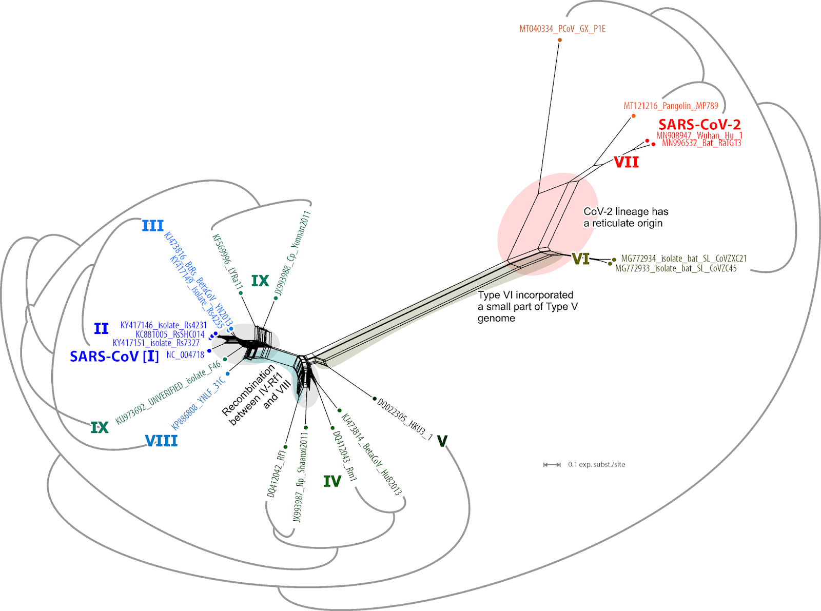
| Fig. 1 A Supernetwork based on 34 individual mitochondrial gene trees (atp1 and atp8 missing due an alignment glitch). Groups (clades) referring to splits not found in any of the gene trees, including the "Septaphyta", are shown in gray font, in blue, groups referring to clades seen in Sousa et al.'s preferred tree. |
Sousa et al.'s set of analyses aimed to filter signal in order to get a better all-inclusive tree, and succeeded to produce support for a "Septaphyta" clade, comprising liverworts and mosses, which is a split not found in any of the inferred (Bayesian) gene trees.
 |
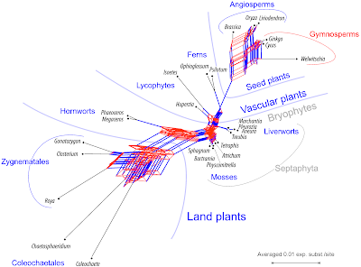
| Fig. 2 Comprehensive but branch-length and frequency ignorant Supernetwork of Sousa et al.'s Bayesian MRC gene trees (trees are provided as supplementary online data on zenodo), inferred from nucleotide sequences. The trees show several alternatives (colored and labeled) regarding the sister lineages of mosses and liverworts. Any split found in at least one gene tree, is represented in this Supernetwork. |
This split did occur, however, when the amino acid sequences were used, instead of the nucleotide sequences.
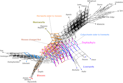 |
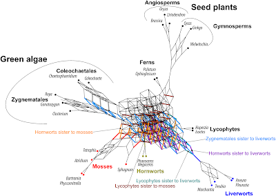
| Fig. 3 Comprehensive branch-length and frequency ignorant Supernetwork of Sousa et al.'s amino acid Bayesian MRC gene trees. The sister taxon of liverworts are either the mosses (= Septaphyta clade) or the outgroup green algae Coleochaete (further inclusive splits include subsequently more outgroups, placing the liverworts as sister to all other land plants). Realized alternatives for mosses include further being a sister of hornworts (in which case liverworts would be sister to higher land plants), or sister to all land plants (brown split: green algae + mosses | rest). |
The alternative to the Septaphyta clade, which does appear in the gene trees, recognizes the liverworts as the closest relative of the vascular plants, while the mosses are resolved as the first branch. As Sousa et al. point out:
The tree inferred from the concatenated nucleotide data set of 36 mitochondrial genes shows mosses as the sister-group to the remaining land plants, as previous analyses of mitochondrial nucleotide data have shown (Liu et al., 2014). ...
The concatenated tree hence only reflects a minor aspect of the Supernetwork (Fig. 1) of the individual gene trees:
... However, the mosses are replaced by the liverworts in the same position when analysing codon-degenerate recoded data.
This seems to be the preferred placement when summarizing the gene trees using the Supernetwork.
In this post, we will take a closer look. Is there a deep, easily obscured signal for the Septaphyta clade in the mitochondria of plants? A signal that only surfaces in some amino acid gene trees (Fig. 2) and the filtered concatenated tree (Sousa et al.'s fig. 2), or is it just a branching artifact?
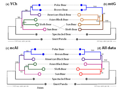 |
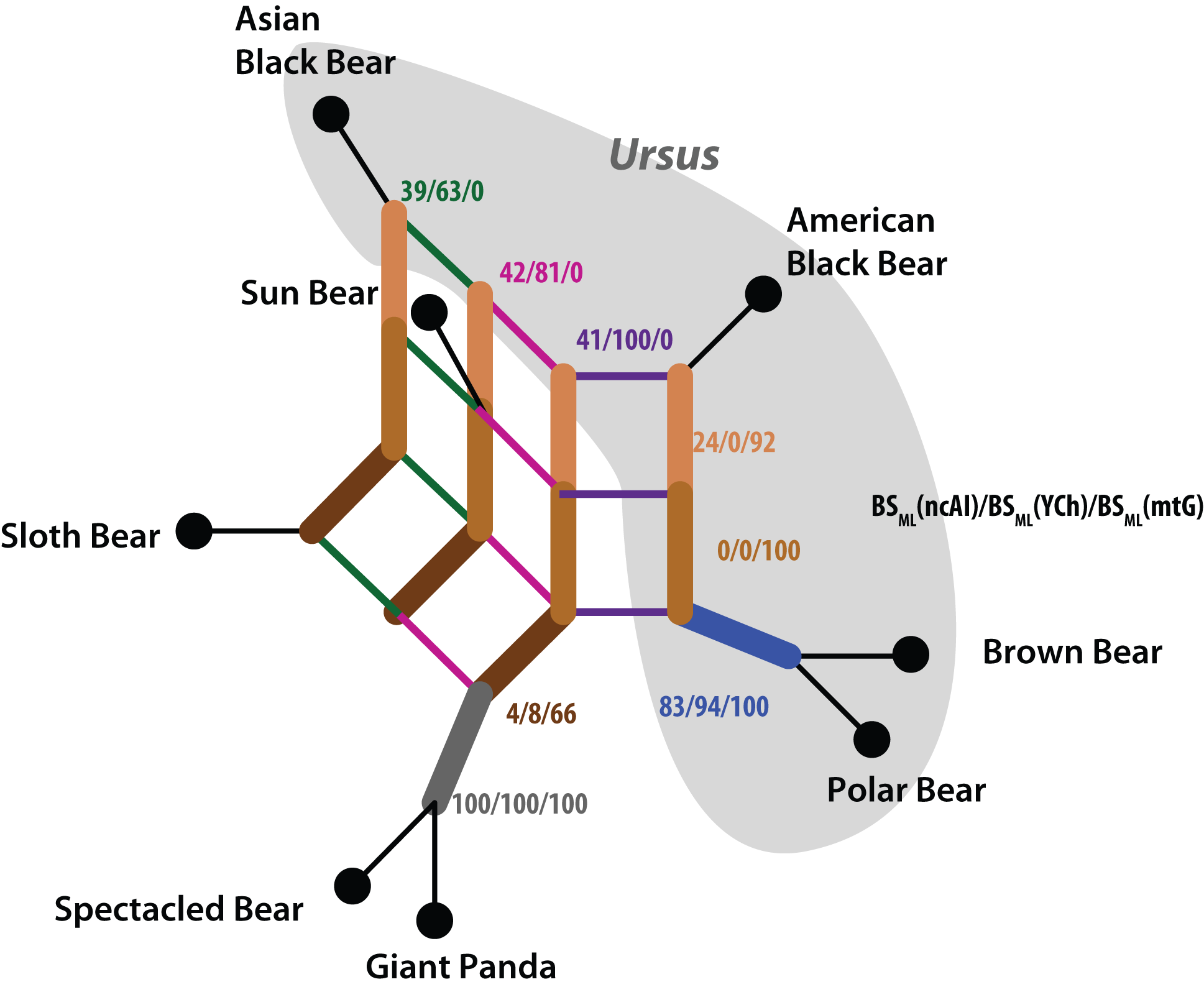
| An example for a (low-supported) artificial clade (cf. Schliep et al., Methods Ecol. Evol. 8: 1212–1220, 2017). The trees in (a), (b) and (c) give the paternal (Y-chromosome), maternal (mt genes) and biparental (nuclear autosomal introns) genealogies. While the paternal and biparental genealogies are compatible (congruent), the maternal is in strong conflict. When combining these three data sets, this substantial conflict decreases branch support and results in the artificial red clade. The support for the artificial clade is low but worrisome: the tips differ substantially from each other and the hypothetical, alternative common ancestors and there are literally no patterns in the data supporting a sister relationship of Sloth and Sun bears. The artificial red clade is a secondary product of the inference: the sister relationship of Polar and Brown Bear is trivial (data and inference wise), the American Black Bear the more likely sister (note the length of competing branches in a/c vs. b). The signal for a clade of Asian Black and Sloth bears is less pronounced, here the mt genealogy clade is strongly incongruent and forces the combined tree to resolve the conflict by introducing the artificial red clade. |
Starting simplyThe Supernetwork in Fig. 1 shows that, no matter which gene we look at, liverworts and mosses were originally most similar to each other, and, absolutely speaking, still close to the (hypothetical) mitochondrion of the ancestor of all land plants. We can illustrate the general situation about the signals using a Neighbor-net inferred from the concatenated data of all 36 genes.
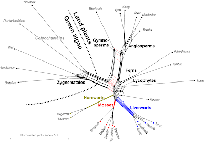 |
| Fig. 4 Neighbor-net based on uncorrected p-distances inferred from the concatenated gene data. |
Note that we used a substitution model via a naive distance matrix for a set of coding genes that include saturated third codon positions. Some phylogenetic relationships are obviously based on trivial signals: the Neighbor-net in Fig. 4 includes ± prominent edge bundles defining neighborhoods in line with generally accepted clades (in bold). To capture these evolutionary lineages (some going back nearly half a billion of years), we just need the raw data but no sophisticated phylogenetic analysis.
In the case of the probably monophyletic gymnosperms, the gymnosperm neighborhood competes with a neighborhood excluding the Gnetidae
Welwitschia, which is the most distinct of the seed plants in this taxon set (this applies to Gnetidae in general, no matter which data are used). In addition, we see a neighborhood defined by the pink edge bundle: a split of green algae +
Welwitschia versus
all other land plants. This is a case of obvious long-edge attraction, enforced (here) by missing data (
Welwitschia lacks data for 12 out of the 34 genes).
The center of the graph with respect to all tips would be a candidate for the ancestral mitochondrion of the common ancestor of all land plants. Closest to this point are the Septaphyta (mosses + liverworts) and the lycophyte
Huperzia (the better represented taxon only missing out on five genes, while
Isoetum miss 15)
.One can depict a phylogenetic hypothesis by just dropping the less pronounced neighborhoods in Fig. 4:
- Most prominent edge bundles define three main cluster (= lineages): green algae, seed plants, and other land plants.
- Within green algae:
- Closterium is sister to Gonatozygon, next is Roya → Zygnematales
- there is no prominent edge bundle connecting Chaetospharidium with the Zygnematales; the closest relative is however the last green algae (→ Coleochatales; only group without a neighborhood).
- Within seed plants:
- Brassica may be the sister of Liriodendron (more prominent edge bundle), Oryza complements the clade as first diverged member → angiosperms
- Cycas is the sister of Gingko, the two are sister to the angiosperms
- this leaves Welwitschia as the first diverged branch.
- Taking the green algae as outgroups:
- the ferns are the sister group of the seed plants (edges longer than the alternative of a primitive land plant clade)
- mosses are sister to liverworts (→ Septaphyta); Huperzia shares the same edge bundle but is apparently sister of Isoetes (→ lycophytes), and the lycophytes appear to be ± primitive sisters of ferns and seed plants
- this leaves the hornworts, a highly coherent group sharing no prominent edge bundles with any other member of the land plant cluster, and hence are a candidate for the first diverging land plant lineage.
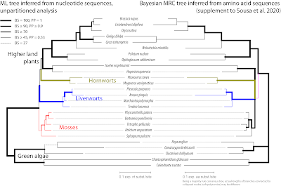
This is a tree hypothesis that is strikingly similar with Sousa et al.'s preferred tree.
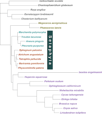 |
| Sousa et al.'s fig. 2 |
The only differences lie in terminal subtrees (
Oryza as sister to
Liriodendron;
Marchantia-Treubia grade,
the position of the latter two within liverworts being unclear based on the Neighbor-net).
Something that is easily overlooked in Sousa et al.'s rooted tree, but that is apparent from the Neighbor-net, is that we should be aware of ingroup-outgroup long-branch attraction (LBA). The green algae are not only highly divergent but also very distant from all ingroup taxa, the land plants.; and the first ingroup branch in Sousa et al.'s tree has the longest root.
Additive and subtractive supportIn principal, when comparing single gene tree samples to combined trees, we face four sorts of signals in our data:
- Very strong signals imprinted in one or a few genes; they will outcompete, and possibly even be re-enforced by any conflicting signal. Walker et al. (PeerJ 7: e7747, 2019), studied this phenomenon for the case of angiosperm plastomes (see also our miniseries The emperor has no clothes on).
- Phylogenetically sorted, weak but consistent signals; they will add up, as branch support will increase with each gene added. In this category fall signals reflecting deep splits obscured by terminal noise, when analyzing a single gene or few genes – like the one found by Sousa et al. supporting a Septaphyta clade.
- Disparate gene histories; eg. because of intergenomic recombination. The support will be diminished with every added gene not sharing the same history.
- General conflict; eg. when combining data from different genomes reflecting different genealogies, such as combining chloroplast (product of biogeographic history) and nuclear data (product of speciation processes) of tree genera. This will be expressed by split bootstrap (BS) support, and may result in artificial clades in the combined/concatenated tree (eg. bear example shown above).
Adding to this is the absence of signal: short-branch culling, a special case of long-branch attraction, which could also explain the inference of a (paraphyletic) Septaphyta clade. If there are few tips in the data that are close (absolute, not only regarding their phylogenetic distance) to the all-ancestor without clear affinities, they may be collected in a subtree, being leftovers from optimizing all other tips with certain affinities and higher distance to the all-ancestor.
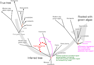 |
| Fig. 5 Short-branch culling. Let's assume liverworts are the sister clade of higher land plants (an alternative with near-unambiguous support from cox1). The signal for this in mitochondrial data is weak (short root). On the other hand, there is a high risk for ingroup-outgroup long-branch attraction (LBA) leading eventually to an artificial Septaphyta clade. Because of (inevitable) LBA, even though the false branch is very short, its support can be high (unambiguous when using Bayesian inference). |
By compiling the support for all alternatives, we can assess where the support is additive or subtractive. We do this using my re-analysis not Sousa et al.'s Bayesian analysis because:
- BS support is more sensitive to internal signal conflict than Bayesian PP,
- to extract this information, we need the tree samples used to establish the branch support.
When doing this, we find that the split defining the Septaphyta clade is not only missing from the nucleotide genes trees but also rarely found in the BS pseudoreplicate samples. Only for seven gene regions (
atp4, atp8, nad2, rpl16, rps2, rps3, rps13) do we find BS ≥ 25; the highest support comes from
rps3 (BS = 65; however, the split is
not found in the corresponding Bayesian MRC of Sousa et al.).
On the other hand, the main alternatives find much higher and more consistent support, as shown here.
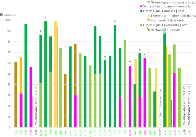 |
| Fig. 6 Competing support for (purple) and against a Septaphyta clade (greens and yellows). Placing the hornworts as sister to all other land plants (pink) is compatible with the hypothesis of a Septaphyta clade as well as the competing alternative of placing the liverworts as sister to higher land plants; note the high support from cox1 gene for an according tree. *, for these genes no hornwort data were included/have been available. |
Short-branch culling, a special form of ingroup-outgroup LBA Now, my BS analyses were deliberately naive, because they did not apply any data partitioning. However, both liverworts and mosses have short-branches while the outgroup, the green algae, are extremely long-branched. If substitution saturation is an issue for misplacing either liverworts or mosses as sisters to all other land plants, then there should also be ingroup-outgroup LBA. A false split of liverwort + outgroup versus the rest, or moss + outgroup versus the rest, has a lower chance to be supported than would a false hornwort + outgroup versus the rest split. The latter directly opens the door for a Septaphyta clade (see Fig. 5).
Let's have a look at the trees of the four genes supporting the Septaphyta split, as the best alternative. ("AA tree/PP" is the amino acid tree provided by Sousa et al.; BS support refers to my unpartitioned ML analyses)
- atp8 — The AA tree is a star tree (comb), strongly distorted by LBA: a Coleochaetales + seed plants | Zygnematales + all other land plants splits has a PP = 1; the short- and long-branched lycophytes are not resolved as sisters.
- rpl16 — Also here, the AA tree is star-like regarding deep relationships: (i) green algae (unresolved), PP = 1; (ii) liverworts, very long root, little internal resolution PP = 1; (iii) mosses (unresolved), root half as long as for liverworts, PP = 1; (iv) higher land plants, short root, PP = 0.88.
- rps3 — No ingroup-outgroup LBA, shortest-branched ingroup, liverworts, resolved as sister to mosses + rest (PP = 0.77); thus, AA tree, not affected by saturation issues, rejects the Septaphyta (PP < 0.23).
- rps13 — Again, the AA tree is star-like, with five tips: (i) green algae (PP = 1); (ii) long-rooted hornworts (PP =1); (iii) liverworts, relatively short root (PP =1); mosses, longer root (PP = 1); (v) higher land plants, shortest root (PP = 0.89).
The Septaphyta root is either extremely short or non-existent, as we would expect for a false clade, because there are no character splits in the matrix that support the taxon split.
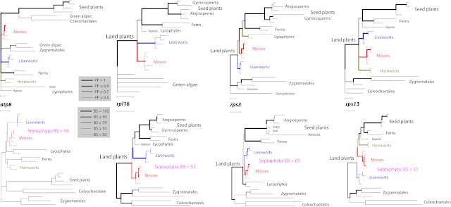 |
| Fig. 7 Sousa et al.'s amino acid Bayesian MRC trees (top row) compared to codon-naive nucleotide ML trees (bottom row) producing highest BS support for a Septaphyta clade. Note that in two cases, rpl16 and rps13, the 'best-known' ML tree shows a competing split with much lower support. |
Typically, since we are looking at a deep split, we would expect that support increases when shifting from (codon-naive) nucleotide to amino acid analysis, because we eliminate terminal noise. However, we observe the opposite (Bayesian PP more easily converges to unambiguous support than BS values). The difference between our codon-naive nucleotide ML and Sousa et al.'s amino acid MRC trees tells us that it is mostly information from the 3rd codon position that triggers a Septaphyta versus the rest split for these four genes — ie. potentially synonymous substitutions that Sousa et al. filtered
against.
Where does the high support comes from for the Septaphyta clade in their combined tree? That tree is based on a matrix, that should have a signal in-between our codon-naive nucleotide and their amino acid analysis.
A five-taxon problem with a glitchSousa et al.'s study is exemplary, in that it provides a careful, and well documented, analysis of the combined data. If you want to infer a potentially good tree, this is one way to do it.
However, their Septaphyta clade is most likely a branching artifact. It still combines data that, genuinely, provides not only diffuse but conflicting information about how the main lineages of land plants diverged from each other (Fig. 6). No analysis, no matter how sophisticated and well-crafted, can compensate for the deficits of the underlying data. By filtering out "noise", one also filters out actual conflicting signal. In this case, this is about how liverworts, mosses, and hornworts stand in relation to the extremely long-branched and divergent outgroup, the green algae, and their increasingly evolved siblings, the higher land plants (lycophytes, ferns, and seed plants). It is another example of what I pointed out in last week's post: Big Data invites big (ie. well supported) errors.
It is important to realize that, although we use many more OTUs, we are still looking at a five-taxon problem. When our data supports one split (or prefers it, being biased or not), there are only three more alternatives to select from.
Ingroup-outgroup LBA draws the hornworts, as the genetically most distinct (longest-rooted) lineage of the "bryophytes", away from liverworts and the lycophyte
Huperzia, which connects the much more diverged higher land plants to the bryophytes. This leaves three alternatives:
- Liverworts are the sister of higher land plants. Their mitochondria show some affinity, but only to the lycophytes, mostly the low-divergent and better sampled Huperzia; and often together with the hornworts, ie. a split incompatible with the hornwort-green algae versus the rest split.
- Mosses are the sister of higher land plants, but their mitochondria show very little affinity to any of them (including Huperzia). In fact, they seem to have the most primitive of all land plant mitochondria.
- Septaphyta are monophyletic, as the trade-off with the least conflict. Being (much) less diverged than the higher seed plants, they are genetically closer, and ± equally close, to the hornworts and the least-evolved higher land plant, the lycophyte Huperzia.
Sousa et al.'s codon-degenerate approach enforced ingroup-outgroup LBA between the hornworts (the worst-sampled ingroup) and the green algae, while decreasing the absolute distance between liverworts and mosses, and increasing their distance to the higher land plants. That is, Alternative 3 outcompetes Alternative 1. Alternative 2 has no support in the data.
Are the mosses sister to all land plants?Probably not. Just because the Septaphyta clade is an artifact, it doesn't mean the Septaphyta cannot be monophyletic — it just means the mitochondrial genes don't provide any clear signal to support or reject such a hypothesis, or any other alternative. The same applies to the mosses as the first diverging lineage; their position in earlier trees is likely also to be an artifact — not a branching, but a data artifact. If their mitochondrial genomes are still very similar to that of the common ancestor of all land plants, then they should be placed like an ancestor in the tree — as a short-branched sister to all of their "offspring", the remaining land plant mitochondria.
Eight of the nine genes that support a moss + outgroup versus the rest split, fail to resolve a moss clade. This is a clear indication that the moss mitochondria are simply primitive (at all gene positions that matter). What divides them from most (or all) other land plants are symplesiomorphies — shared but ancestral sequence patterns. The only gene that prefers both splits at once, mosses as sister to all other lands plants as well as a moss clade, is
nad4 (BS = 67 and 62, respectively); but only when using nucleotides.
 |
| Fig. 8 A small but important difference: the codon-naive ML nucleotide (nt) tree (left) shows a moss clade as sister to all other land plants. The Bayesian amino acid (aa) MRC tree for the same gene shows a wrong split (purple internode) between green algae + ferns + angiosperms (long-branch, prominent roots) and bryophytes + lycophytes (mostly short-branched, short roots). By translating nucleotides into amino acids one may eliminate genuine discriminative signal encoded in synonymous substitutions, while in other, faster evolving parts of the tree, the same site/gene is oversaturated/biased. The poorly supported sister relationship of Roya and Gonatozygon within the green algae in the nt ML tree is an artifact, correctly resolved by the aa tree based on the same gene. |
The shift from nucleotide data (ML / BS) to amino acid data (Bayesian MRC) triggers ingroup-outgroup LBA between green algae and ferns + seed plants (PP = 0.53; 'short-branch culling' of bryophytes and lycophyte
Huperzia), and results in a branching artifact — the monophyly of higher land plants is well established, and hence they should form a clade.
By contrast, the genes providing strong support for a moss clade (such as
atp1, atp8, ccmB, cob, cox1, cox3, nad2, nad5, rpl6, rpl16, rps3, rps13, and
rps14) fail to resolve any deep relationships at all, or prefer different alternatives (including the Septaphyta hypothesis:
atp8, rps3, rps13). The combined tree's solution is therefore a least-conflicting one, again — a moss clade (based on a consistent signal in the majority of genes: 13 with BS ≥ 90; in total 24 with BS ≥ 58) as sister to the rest of the land plants (based on a signal found in other genes not reflecting the monophyly of mosses). This solution adds to the phenomenon that moss mitochondria are generally primitive (ie. show a variant basically ancestral to all other land plants), and doesn't conflict with a wide range of otherwise conflicting splits strongly supported by individual genes (in contrast to the Septaphyta clade, see Fig. 6).
Conclusion Having spent some time with the data and gene trees, I have little hope that mitochondrial data can be used to resolve the deep relationships between land plants. Each tweaking may result in something different, and the support-after-tweaking will be inflated.
Nevertheless, it will be worthwhile to close the data gaps, especially for the hornworts. This may not solve the 5-taxon problem,* but may give unique insights in how the mitochondrial genome evolved and sorted during the initial radiation of land plants.
Notably, the mitochondriomes of land plants can differ in the arrangement of their genes; which means that they recombined with or within the nucleome (or even plastome). While in some plants the mitochondriome is passed on via both parents (like in
Ginkgo or
Cycas), in others it is only the mother (most, maybe all, angiosperms). Plants may have colonized land more than once, and expanded quickly, so that lineage crossing and also lineage sorting may be an issue — marine species can be cosmopolitan
and genetically heterogeneous (cryptic speciation). Thus, some mitochondrial genes may tell different stories from others. Instead of trying to solve which of the alternatives is correct (which is what most phylogenetic literature revolves around), we should find out which gene or part of the genome agrees with which alternative, as they may be all true.
The question to address with mitochondrial data cannot be whether mosses, liverworts or hornworts are the first diverging branch of extant land plants, but should be why moss, liverwort and hornwort mitochondriomes show different stages of evolution, as exemplified by the
nad4 trees in Fig. 8.
Data availabilityAn archive including the support consensus networks (in Splits-N
EXUS format) and inferred gene ML trees (plain N
EWICK), as well as the comprehensive split support table (XLSX format), has been uploaded to
figshare.
* It may help to have an in-depth analysis of a more focused taxon set with no data gaps that minimizes the risk of LBA. This starts with a better selection of taxa representing the higher land plants:
- Oryza (the rice) is a domesticated, much cultivated, and thus extremely evolved and polyploid monocot. If there is any deep signal embedded in the mitochondria of seed plants, the mitochondrion of rice is probably the last place to look for it.
- When trying to resolve the deepest land relationships, including a Gnetidae like Welwitschia (a genus that is an evolutionary oddball to start with), makes equally little sense — like any of the three surviving genera of this unique gymnosperm lineage, it is genetically the outer-most tip of an iceberg. Each mutation in its genome is the product of an unknown number of divergences in the past.
- If any seed plant should be included at all, would be more than sufficient to have: Liriodendron, a magnoliid, and thus a member of the least-diverged angiosperm lineage, plus Cycas, as a representative of an ancient, slow-evolving gymnosperm lineage. These are much more recent additions to the plant Tree of Life.
- Being a tip of an iceberg applies even more to Isoetum. It is strikingly similar only to the other lycophyte, but it has more data gaps and is much more diverged, and thus can invite branching artifacts. When one wants to dig deep, the much more primitive Huperzia is obviously the better representative.
- Last, the green algae are the only possible outgroups for inference, but they are poor for this – apparently, their mitochondria have evolved much farther from the common ancestor than those of the land plants. Rather than inferring trees including them, one should infer trees without them, and then optimize their position within trees that will then potentially be unbiased by outgroup-LBA — eg. using the evolutionary placement algorithm, to test the land plant root. An interesting experiment could also be to infer the sequence of the common ancestor(s) of modern-day green algae (lacking a time machine to sample it), and use them instead. The new RAxML-NG, for example, allows for ancestral state reconstruction of nucleotides.
In addition, standard 4-base substitution models are not the best choice when analyzing matrices with a high proportion of ambiguous base calls, like Sousa et al.'s codon-degenerate matrix (note that Sousa et al. already applied models that compensate for substitutional bias). This is especially so, given the importance of synonymous mutations to resolve relationships in the slow-evolving lineages, and slow evolving genes. One could try to use ambiguity-aware substitution models instead. The newest releases of RAxML-NG (
Kozlov et al. 2019, Bioinformatics 35: 4453–4455) include models for "phased" and heterozygous data — ie. models that can make use of ambiguity codes as additional information during tree inference (see also
Potts et al. 2014, Syst. Biol. 63:1–16).