Topological restrictions: some comments


In a recent post (Different topological restrictions of rooted phylogenetic networks. Which make biological sense?), Leo and Steven synthesized a lot of the issues that have been raised in recent years, both in this blog and in the literature, about the underlying models for rooted phylogenetic networks. This is an excellent summary (and explanation) of the current situation; please read it if you have not already done so.

The key issue for biologists is: what are we trying to model biologically? In one sense the answer is trivial: "evolutionary history". However, this answer is uninformative, in the sense that it is too broad to be practical. We do not know enough about evolutionary history for it to be obvious which model(s) we should use, and we presumably never will know (we were not there to study it, and it happens too slowly to study it now).

Nevertheless, we need to make decisions about models, and in many cases quite detailed decisions. Therefore, we need public discussion about the various possible models that have been suggested, as well as suggestions for new models. Unfortunately, the impetus for this has almost always come form the computational side rather than the biological side, if only from practical necessity — a mathematician cannot proceed without a model. (A biologist can't either, but they seem to be much more comfortable with vague word models rather than quantitative mathematical ones.)

So, I will provide an initial response to Leo and Steven's points, as a staring point for discussion, in the order in which they raised them. Hopefully, someone else will have something to say, as well.

Rooted

If there is assumed to be a single origin of life, and evolution is assumed to be acyclic, then there will always be at least one root in every evolutionary network. Indeed, if we are studying a monophyletic group of organisms then there will always be precisely one root. But if we are studying a polyphyletic group then technically there are multiple roots, in the sense that we cannot reconstruct the most recent common ancestor of the group. In practice, we have ignored this issue, and simply reconstructed the ancestor anyway, as best we can, since that is what the current tree-building algorithms do. In this sense, the only difference between an evolutionary tree and an evolutionary network is the complication caused by horizontal gene transfer, in which we might consider a species' genome to be polyphyletic, as well.

So, a single artificial root will probably suffice — see Steven's earlier comment: "the multiple-root situation can probably be reduced to the single-root situation by having some kind of high-degree (i.e. unrefined) artificial root which is the parent of the real roots."

Acyclic

Acyclicity is an obvious criterion for evolution, because a descendant cannot be its own ancestor. So, in a network we should treat this as "sacred" — an evolutionary network in its final form cannot show any directed cycles.

This does not, I guess, preclude algorithms that do not themselves require acyclicity, as biology always violates mathematical assumptions (eg. normality, homoscedasticity, etc). However, I think that we should require the output to be acyclic.

This is not necessarily an issue for reconciliation between gene trees and species trees, as raised in the original blog post. In this scenario the resulting phylogeny is a tree, and therefore cannot show cycles, by definition.

Time-consistent

Time consistency is a stronger form of acyclicity, in the sense that the acyclic parts of a network are also restricted by time's arrow. It is another obvious criterion for evolution, because a descendant cannot reticulate with its predecessors.

However, this requirement is confounded by incomplete taxon sampling, as noted by Leo and Steven. To deal with this, we can allow "ghost" lineages representing hypothesized missing taxa. This does, nevertheless, raise the issue of where we draw the line. Any two trees can be reconciled by allowing enough ghost lineages, just as is done by algorithms for the gene duplication-loss problem, where minimizing the numbers of unobserved duplications and losses is the optimality criterion. Similarly, how many ghost lineages should we allow in a reticulating network? Perhaps we should be minimizing them, too.

There is also the more fundamental issue of whether time-consistency should actually be a requirement at all. It has been pointed out a number of times that this is not a requirement for anthropology, for example, where transfer of non-genetic information through time is not only possible but quite common. This has been discussed in earlier blog posts.

So, in a general sense we cannot make time consistency a mandatory requirement of evolutionary networks. However, we could do so for strictly biological networks, where information transfer occurs with gene flow, which must follow time's arrow.

Degree-restricted

Nodes with indegree 1 and outdegree 1 are usually considered to be unnecessary, because they do not represent anything more than would an edge (or arc). The only times they have been seriously suggested are when placing known fossils onto a tree, and the fossil is claimed to represent an ancestor of one of the nodes. However, this is considered to be inappropriate, because we can never be sure that any specified fossil is actually an ancestor, as opposed to being a sister to one of the ancestors (see the blog post at Evolving Thoughts).

Indegree >2 has also been considered to be problematic in phylogenetics. If a sexually reproducing organism has two parents, then theoretically we cannot observe indegree>2. In practice, however, evolutionary events may occur over a short enough time-scale that we cannot distinguish a series of individual indegree-2 events, so that for practical purposes a network might end up showing indegree >2. This is analogous to "soft polytomies" in trees, where outdegree >2 represents uncertainty.

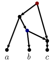
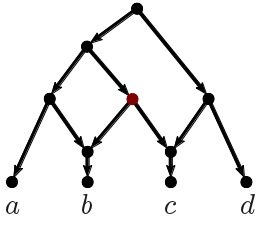
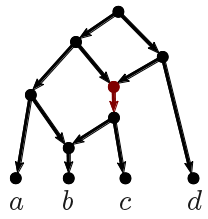
Tree-child, Tree-sibling, Reticulation-visible

These network restrictions all refer to so-called "invisible" nodes (nodes from which all paths end up in reticulations). All nodes in a tree are visible, and so there is no analogous situation in tree-building from which we might derive a response (as I have done several times above).

The basic issue with invisible nodes is restricting their occurrence. Theoretically, we could add an infinite number of invisible nodes to a network, but few, if any, of them would be based on any inference from the data. So, tree-child networks ban them entirely, whereas tree-sibling and reticulation-visible networks allow them under particular circumstances.

It is difficult for me to see exactly how I should interpret invisible nodes biologically. How can I reconstruct their features, for example? Invisible nodes tend to appear when combining multiple trees into a network, and so they are not usually constructed directly from character data. Biologically, they might exist, but there seems to be little reason to consider them as well-supported inferences, as we do for visible nodes.

In this sense, they have much more of the feel of mathematical artifacts than do visible nodes.

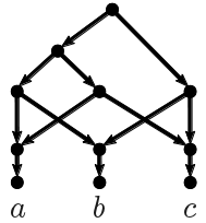
Galled trees, Galled networks, Level-k

These are all artificial restrictions on networks that do nothing more than limit the complexity (and thus make the algorithms more tractable). There seems to be no good biologicals basis for using any of these criteria as restrictions (as opposed to using them as network descriptors).

There is, however, a good logical basis for their use — simpler networks are to be preferred over more complex ones, at least as working hypotheses for evolutionary history. The problem with this attitude seems to be that sometimes simpler networks look less biologically realistic than do more complex ones (eg. level-1 networks might spread the reticulations across the network whereas level-3 networks can concentrate them in one place).

Regular and normal

These always seem to me to be of mathematical interest for characterizing networks, rather than being of any biological interest. But maybe that is just my ignorance.

Directed Acyclic Graph or tree-with-edges-added?

To me , this is one of the BIG questions. Until biologists come to grips with this, I do not see how the computational people are going to make the helpful contributions that they obviously desire (or, at least, the ones I know). I have thought (and read) about this a lot, and I have come to the (perhaps unfortunate) conclusion that the answer is: "both".

From the mathematical point of view, the problem is simply that certain network topologies will not be considered when we add reticulation nodes to a tree. So, we automatically exclude those topologies if our algorithm starts with a tree. From the biological point of view, the issue is whether we consider evolutionary history to be approximately tree-like or whether it is fundamentally reticulated.

My reading of the literature is that those people dealing with hybridization in eukaryotes are leaning towards the "tree obscured by vines" model, whereas those dealing with horizontal gene transfer in prokaryotes prefer the "anastomosing plexus" model. Perhaps it is too soon to tell whether this dichotomy will continue; but, certainly, discussion about the hybridization issue goes back to the early 1980s, and since then the opinion about the fundamentally tree-like nature of history has been repeatedly expressed. Moreover, those people using reduced median networks and median joining networks for mitochondrial data seem to be interested in simplifying their initially complex network as much as possible, and then interpreting the resulting network in terms of a few conflicting parsimony trees; I interpret this as a preference for trees over networks.

Of course, preferring a reticulated tree model may just be historical inertia, whose importance in the daily lives of scientists should not be underestimated.

Different topological restrictions of rooted phylogenetic networks. Which make biological sense?


Those readers active in the field of evolutionary phylogenetic networks will know that there are many different definitions ofrooted phylogenetic networkin circulation. While certain features are almost universal (e.g. rooted, acyclicity), many are not. Why do these differences arise? There are multiple answers to this. Some arise because of differing opinions on what biologically realistic is, and (relatedly) what the correct balance is between biological detail and mathematical abstraction. Others arise because they make optimization problems on networks easier to solve. This should not automatically be viewed as mathematics prescribing reality to biology, but rather as the observation that if evolution looks like this then certain optimization problems can be solved well. Finally, some differences are superficial; they do not lead to any intrinsic differences in the model or its underlying mathematical structure. Of course,superficialis highly context dependent, as some of the examples below will show.

Here we list some well-known and less-well known properties that have surfaced in definitions of rooted phylogenetic network. We will take as given that evolution is directed i.e. that the arcs in the network have an explicit orientation (representing the flow of time). Below most properties we show a figure of a network violating it.

The question to our readers, particularly those from the biological side of the spectrum: which of the following properties make sense? And which other restrictions would make more sense biologically?

Rooted
A root is a node with indegree 0, meaning that it does not have any ancestors. If evolution is assumed to be acyclic (see below) then there will always be at least one root. Most articles writing about rooted phylogenetic networks assume a single root (which is necessarily an ancestor of every node in the network). Some time ago on this blog David raised the question of whether it would not sometimes be better to allow multiple roots. This is an interesting point both from the perspective of interpretation (what does it mean?) and its impact on algorithmic efficiency.

Acyclic
Most models assume acyclicity: it is not possible to walk along the arcs of the network (respecting their orientation) such that you end up back where you started. The most intuitive argument for this is the passing of time: if arcs represent forward motion through evolutionary time, how can you end up back at an earlier point in time? Recently someone pointed out to me that in the reconciliation literaturewhere one shows how to reconcile a given gene tree with a given species treeacyclicity is actually not sacred at all. The reason for this is that, without the acyclicity constraint, the problem becomes computationally tractable. See this recent RECOMB 2013 article [3] for an example of this.

Time-consistent
This is an interesting property. It was introduced to prevent reticulation events between non-contemporaneous taxa. That is, to avoid absurd situations such as an organism hybridizing with its ancestor. The most common mathematical articulation of time-consistency is this: it should be possible to put atime-stampon each node of the network such that (a) time always moves strictly forward along tree-edges , and (b) all the nodes involved in a reticulation event have the same time-stamp. The figure here shows a network that is not time-consistent. For many contextualisations ofreticulation eventtime-consistency seems to make a lot of sense. But there is a catch. A network might fail to be time-consistent only for the rather artificial reason that we failed to sample a taxon that was, in fact, part of the network (incomplete taxon sampling). Given the reality of incomplete data, demanding time-consistency might be too prohibitive. However, as with all restrictions in this blog, it is perhaps useful as a selection criterion for preferring one network over another.

Figure 1: A network that is not time-consistent. The red and blue node are the two parents of a reticulation node but cannot have coexisted in time.


Degree-restricted
The indegree of a node is the number of parents of it, and the outdegree of a node is the number of children of it. In a bifurcating, rooted phylogenetic tree all nodes have indegree-1 (except the root: indegree-0) and outdegree-2. Polytomies have outdegree-3 or higher.  In a rooted phylogenetic network we also have reticulation nodes i.e. nodes with indegree-2 or higher. Articles differ in the degree-restrictions they place on nodes; there is an entire zoo of different permutations possible. Many articles agree that nodes with indegree-1 and outdegree-1 should not be allowed, because they are phylogenetically uninformative (and indeed such nodes are also rarely encountered in the phylogenetic tree literature). But what about polytomies? And what about reticulation nodes: should they be permitted to have indegree-3 or higher, and if so how should such “reticulate polytomies” be interpreted? From a parsimony perspective it is usual to argue that reticulate polytomies should be more “expensive” than indegree-2 reticulations, because a single reticulation polytomy can explain far more discordance than a single indegree-2 reticulation. Interestingly, some optimization problems are not really affected at all by degree-restrictions on phylogenetic networks (e.g. the hybridization number problem) while others are highly sensitive to degree-restrictions (e.g. the small parsimony problem).

Tree-child
Every node has at least one non-reticulate child. This restriction makes sure that there are no "invisible nodes", i.e. nodes from which all paths end up in reticulations. As a result, this restriction makes many computational problems more tractable and mathematical reasoning easier. For example, consider the basic Tree Containment problem, i.e. given a phylogenetic network and a phylogenetic tree, decide if the network displays the tree, see [8]. This problem was shown to be tractable for tree-child networks, while it is NP-hard for most other classes of networks (time-consistent, tree-sibling, regular). This seems important because if it is already hard to tell if a given tree is in a given network, then it seems  a daunting task to try to build networks of that class from any kind of data.

It should be noted that there is of course no guarantee that "real" evolutionary histories are tree-child. In fact, simulation studies show that only under very low recombination rates one can expect tree-child networks [1][2].

Figure 2: A network that is not tree-child. The red node does not have a non-reticulate child.

Tree-sibling
Every reticulate node has at least one non-reticulate sibling. Originally introduced by Cardona, Llabrés, Rosselló and Valiente who write "Biologically, this condition means that for each of the reticulation events, at least one of the species involved in it has also some descendant through mutation" and showed that networks can efficiently be compared (with a polynomial-time computable metric) if they are both tree-sibling and time-consistent.

An advantage of the class of tree-sibling networks is that it is much larger than the class of tree-child networks. If a reticulation has no non-reticulate siblings, then its parents have no non-reticulate children. Hence, every tree-child network is tree-sibling. However, it can easily be seen that there are many tree-sibling networks that are not tree-child. Computationally, the tree-sibling restriction does not seem to help as much as the tree-child restriction. Again, there is no guarantee that the "real" network is tree-sibling, but it might be more likely, see [1][2].

Figure 3: A network that is not tree-sibling (the red node does not have a non-reticulate sibling).

Reticulation-visible
From every reticulation node there is a path to some leaf or cut-arc (a branch whose removal disconnects the network) such that this path does not pass through any reticulations. This is another attempt to weaken the tree-child restriction, thus obtaining a larger class of networks for which many computational problems are still tractable. It is incomparable with tree-sibling (a reticulation-visible network does not have to be tree-sibling and vice versa) but this class clearly contains the class of tree-child networks, and in fact is much larger. It does not forbid all invisible nodes, but just invisible reticulation nodes. It has been shown in the book by Huson, Rupp and Scornavacca that the so-called Cluster Containment problem becomes tractable for reticulation-visible networks. If the same is the case for the Tree Containment problem is still an open question.

Figure 4: A network that is not reticulation-visible. The red reticulation node is not "visible".

Galled trees
All reticulation cycles are disjoint. Introduced by  Gusfield, Eddhu and Langley [6] although studied before under different names. Makes computational problems much easier but seems biologically unrealistic. On the other hand, galled trees could have a future in the context of data-display networks, by using the galls to show where the reticulate activity is in the network, rather than claiming that each gall represents exactly one reticulation event.

Galled networks
Each arc leaving a reticulation node is a cut-arc. Introduced by Huson and Klöpper [7] (who gave a different but equivalent definition) as a generalization of galled trees, giving a fast algorithm for constructing galled networks from clusters. Hasn't been studied much since. (Be aware that there is also an article using "galled network" as an alternative term for galled tree.)

Figure 5: A network that is not a galled network. The red arc leaves a reticulation node but is not a cut-arc.

Level-k (not a restriction, but a measurement)
Also a generalization of galled trees (which are basically level-1 networks). Every network is a level-k network for some k. Hence, “level-k” should not really be viewed as a topological restriction, but rather as a measure of how “tangled” (intensely concentrated) the islands of reticulation are in the network. The higher k is, the more tangled the network is; level-0 networks are simply trees. For more information, see a previous blog. Other proposed measurements of tangledness include k-nested, r-reticulation and depth-k.

Regular and normal
If you see a phylogenetic network as a representation of a set of clusters, then it makes sense to consider regular networks (introduced by Baroni, Semple and Steel). A network is regular if it is the so-called "cover digraph" (Hesse diagram) of its set of clusters. Hence, for each set of clusters, there exists a unique regular network with precisely that set of (hardwired) clusters. Normal networks have the additional requirement of being tree-child, thus forming a very restricted class of networks. For example, the network in Figure 1 is not regular and hence also not normal.

DAG or tree-with-edges-added?
This is a rather subtle one. If one views a phylogenetic network as a tree with edges added, then this leads to a different space of networks than the “a phylogenetic network is essentially a directed acyclic graph” definition encountered in other articles. The point being that if you insist that a network has to be “grown” from some tree starting point (by adding edges in a certain way), certain topologies cannot be reached which can be reached if the we do not anchor it in this way. The following figure shows an example.

Figure 6: A network that cannot be obtained by adding edges to a tree (for common edge-adding rules).

It can be shown that any tree-sibling network can be constructed by adding edges to a tree, but the network in Figure 3 shows that the converse is not true (the shown network can be constructed by adding edges to a tree, but is not tree-sibling). 

This restriction touches on the fundamental question whether there exists something like a species tree, and if it might be possible to reconstruct this species tree before starting network analysis.


A related but stronger (?) restriction was recently used by Wu [9]. In his RECOMB 2013 article, he writes “(R1) For a network N, when only one of the incoming edges of each reticulation node is kept and the other is deleted, we always derive a tree T'.”

Conclusion
We see from this list that there are already some quite different topological properties and restrictions in circulation for rooted phylogenetic networks. To biologists these discussions might appear to be a strange side-show to keep computer scientists in work. But it runs deeper than that, because it touches on three fundamental issues. Firstly, what are we trying to model exactly? Secondly, the importance of understanding the networks that your favourite software for constructing rooted phylogenetic networks will not build, however biologically relevant, due to the fact that they are a priori excluded from its search space. Finally, since the total number of networks is huge, it could be inevitable to focus on certain restricted classes of networks when one wants to search through network-space efficiently.

Note: There is a follow-up post Topological restrictions: some comments.

REFERENCES

[1] Miguel Arenas, Mateus Patricio, David Posada and Gabriel Valiente. Characterization of Phylogenetic Networks with NetTest. In BMCB, Vol. 11:268, 2010. 

[2] Miguel Arenas, Gabriel Valiente and David Posada, Characterization of Reticulate Networks Based on the Coalescent with Recombination, Mol Biol Evol (2008) 25 (12):2517-2520.

[3] Mukul S. Bansal, Eric J. Alm, Manolis Kellis, Reconciliation Revisited: Handling Multiple Optima when Reconciling with Duplication, Transfer, and Loss, RECOMB 2013.

[4] Gabriel Cardona, Merce Llabres, Francesc Rossello, Gabriel Valiente, The comparison of tree-sibling time consistent phylogenetic networks is graph isomorphism-complete, arXiv:0902.4640 [q-bio.PE], 2009.

[5] Gabriel Cardona, Mercè Llabrés, Francesc Rosselló and Gabriel Valiente. A Distance Metric for a Class of Tree-Sibling Phylogenetic Networks. In BIO, Vol. 24(13):1481-1488, 2008.

[6] Dan Gusfield, Satish Eddhu and Charles Langley. Efficient reconstruction of phylogenetic networks with constrained recombination. In CSB03, Pages 363-374, 2003.

[7] Daniel H. Huson and Tobias Klöpper. Beyond Galled Trees - Decomposition and Computation of Galled Networks. In RECOMB 2007, Vol. 4453:211-225 of LNCS.

[8] Leo van Iersel, Charles Semple and Mike Steel, Locating a Tree in a Phylogenetic Network, Information Processing Letters, 110 (23), pp. 1037-1043 (2010).

[9] Yufeng Wu. An Algorithm for Constructing Parsimonious Hybridization Networks with Multiple Phylogenetic Trees. RECOMB 2013.

An open question about computational complexity


This is a guest blog post by:

Jesper Jansson

Laboratory of Mathematical Bioinformatics, Kyoto University, Japan

Here is an open problem for people interested in computational complexity issues related to phylogenetic networks.

In a recent paper we introduced a parameter called the "minimum spread" that measures a kind of structural complexity of phylogenetic networks:
T. Asano, J. Jansson, K. Sadakane, R. Uehara, G. Valiente (2012) Faster computation of the Robinson-Foulds distance between phylogenetic networks. Information Sciences 197: 77-90.

The definition is as follows:
  • The "minimum spread" of a rooted phylogenetic network N is the smallest integer x such that the leaves of N can be relabeled by distinct positive integers in a way that at every node u in N, the set of all leaf descendants of u forms at most x consecutive intervals.
For example, any phylogenetic tree has minimum spread 1 because if we do a depth-first traversal of the tree and number the leaves in the order that they are discovered, then at each node, the set of leaf descendants corresponds to a single consecutive interval. This property was used in, for example, Day's algorithm from 1985 for comparing phylogenetic trees and constructing a strict consensus tree.

Similarly, any level-k phylogenetic network has minimum spread at most k+1 (see our paper for the proof). Moreover, any "leaf-outerplanar network" has minimum spread 1, where a "leaf-outerplanar network" is a network that admits a non-crossing layout in the plane with the root (if any) and all leaves lying on the outer face. Today's existing software typically outputs such networks. So, for certain classes of phylogenetic networks, we automatically get a nice upper bound on the minimum spread.

Having a small minimum spread means that the phylogenetic network is "tree-like" in the sense that its cluster collection has a space-efficient representation. But are compact representations of the clusters in a network useful?

Well, they can be employed to compare phylogenetic networks quickly, for example when using the Robinson-Foulds distance to measure the dissimilarity between two phylogenetic networks. There may be other applications, too. On the other hand, if a phylogenetic network is "chaotic" and non-tree-like then the minimum spread will not be a helpful parameter when looking for a compact encoding of its branching information.

At this point in time, not much is known about how to compute the minimum spread efficiently. As an example, consider the class of level-k networks for any fixed k > 1. According to Lemma 6 in our paper, we can always find a leaf relabeling function that yields spread at most k+1 in linear time, but that might not be the minimum possible for some particular level-k network.

As observed by Sylvain Guillemot and Philippe Gambette (independently of each other), a related result for the k-Consecutive Ones Problem implies that computing the minimum spread of an arbitrary phylogenetic network is NP-hard in the general case, although we can expect it to be easier when restricted to special cases:
P. W. Goldberg, M. C. Golumbic, H. Kaplan, R. Shamir (1995) Four strikes against physical mapping of DNA. Journal of Computational Biology 2: 139-152.

In summary, the following is still open:
  • What is the computational complexity of computing the minimum spread when restricted to particular classes of phylogenetic networks?

Are mathematical constraints biologically realistic?


Mathematicians and other computational scientists have produced their own definitions of phylogenetic networks, independently of biologists. For the evolutionary type of phylogenetic network, the definition usually looks something like this:

A phylogenetic network is a rooted, directed graph (consisting of nodes, plus edges that connect each parent node to its child nodes) such that:
(1) There is exactly one node having indegree 0, the root
        - all other nodes have indegree 1 or 2
(2) All nodes with indegree 1 have outdegree 2 or 0
        - nodes with outdegree 2 are tree nodes
        - nodes with outdegree 0 are leaves, distinctly labelled
(3) The root has outdegree 2, and
(4) Nodes with indegree 2 have outdegree 1, called reticulation nodes.

An obvious question of interest is how (or whether?) this definition connects to what biologists have in mind when they use the term "phylogenetic network". Clearly, this definition places considerable restrictions on the networks that will be inferred by any mathematical algorithm, which in turn affects their use as models for biological inference.

The first thing to note is that unrooted networks are excluded, because the graph is directed. Thus, many (if not most) of the phylogenetic networks that have appeared in the literature are excluded from the discussion. Furthermore, a tree is considered to have all internal nodes with indegree 1 and outdegree 2 (i.e. no reticulation nodes), and we know this to be biologically unrealistic, in general. (Otherwise, this blog would be redundant!)

Biologically, the other parts of the definition imply:
One node of indegree 0
- the network has no previous ancestry that is to be inferred
Nodes with outdegree 0 are labelled
- observed (contemporary) taxa occur only at the leaves
All nodes with indegree 2 have outdegree 1
- reticulation and speciation cannot occur simultaneously
No nodes with indegree >2
- reticulation events cannot involve input from more than 2 parents simultaneously
No nodes with outdegree >2
- speciation involves only two children at a time.

These do not appear to be onerous biological restrictions. Indeed, he first two have been standard characteristics of tree-building for several decades. The other three are also logical extensions of  the restrictions that have previously been placed on trees. However, phylogenetic history is unlikely to have been as simple as implied by these features. Thus, biologists will need to keep a careful eye on whether the simplifications are affecting the networks inferred for their particular group of organisms.

Other restrictions

In addition to the restrictions created by the definition, other topological restrictions have been used to make the mathematical inference algorithms computationally tractable. Thus, only certain sub-families of possible networks are considered by most of the computer programs. These include:
  • tree-child network, tree-sibling network
  • level-k network, galled tree
  • binary input trees for hybridization and HGT networks
  • binary characters for recombination networks.
These restrictions may be unrelated to each other; so, we can consider them separately.

Tree-child, Tree-sibling

In a tree-child network, every internal node has at least one child node that is a tree node
- ie. a reticulation event cannot be followed immediately by another reticulation event
In a tree-sibling network, every reticulation node has at least one sibling node that is a tree node
- ie. a parent cannot be directly involved in two separate reticulation events
Note that every tree-child network will also be a tree-sibling network, but not vice versa.

Algorithmically, these two restrictions may involve the addition of extra tree nodes to an inferred network, in order to satisfy the restrictions. Biologically, the question is whether real networks are this simple. Arenas et al. (2008) simulated data under the coalescent with recombination, and found that even at small recombination rates most of the networks produced were already more complex than a tree-sibling network. On the other hand, Arenas et al. (2010) analyzed real population-level data from the PopSet and Polymorphix databases using the TCS program, and found that >98% the resulting networks could be characterized as tree-sibling. So, there is cause for optimism, in the sense that the "optimum" networks algorithmically are not necessarily complex, at least for closely related organisms (ie. within species).

Level-k network, Galled tree

A network has level k if each tangled part of the network (ie. each biconnected component) contains at most k reticulation nodes (see this previous post). This is a generalization of the older notion of galled trees, in which reticulation cycles do not overlap (ie. do not share edges or nodes), as galled trees are level-1 networks. Level-k networks can also be seen as a generalization of networks with k reticulation nodes, although there may be a difference between a network with minimum level and one with a minimum number of reticulations.

Algorithmically, these restrictions have been used to guide the search for (or choice of) the "optimal" inferred network. Biologically, these notions do not seem to have been investigated, but basically they restrict how complex inferred reticulation histories can be. In particular, they restrict the complexity of any given subset of each network. It has been noted that optimizing k can easily lead to networks that look biologically unrealistic (Huson et al. 2011).

Binary input

The requirements for binary input trees and binary characters are restrictions that have been applied in the past, because they greatly reduce the complexity of the input to the network algorithms, but they are now being relaxed. Effectively, the restrictions are to fully dichotomous trees and SNP characters. These are not unusual restrictions in evolutionary analysis, but they are obviously unrealistic.

As I noted in an earlier blog post, non-binary data often reflect uncertainty in the input, rather than a strictly bifurcating history, and this is not taken into account in the network inference if the input is restricted to a binary state. In particular, it may be unnecessarily hard to construct a network (because not all of the data signals relate to reticulation), and the resulting networks may have far too many reticulation nodes.

Conclusion

It is still an open question about the extent to which we can use these topologically restricted families of mathematical networks as a basis for reconstructing biological histories. Clearly, much more work is needed to understand the connections between the mathematical restrictions and the requirements of biological modelling.

References

M. Arenas, M. Patricio, D. Posada, G. Valiente (2010) Characterization of phylogenetic networks with NetTest. BMC Bioinformatics 11: 268.

M. Arenas, G. Valiente, D. Posada (2008) Characterization of reticulate networks based on the coalescent with recombination. Molecular Biology and Evolution 25: 2517-2520.

D. H. Huson, R. Rupp, C. Scornavacca (2011) Phylogenetic Networks: Concepts, Algorithms and Applications. Cambridge University Press.