A sneak peek into the upcoming SplitsTree 5


For some time now, the official SplitsTree page (www.splitstree.org) has been offline. The reason is that a major update is on the way: SplitsTree5. A beta version is already available, so let's take a quick look at it.

During installation you will be asked how much RAM you want to dedicate. Give as much as possible, in case you want to handle large tree with myriads of splits. I chose 16 GB (ie. half of the RAM installed on my PC).

Here's how it looks when you start the program:


The menus known from SplitsTree4 are still there, and the important functions appear to be already implemented. Some are new, and some have been moved:
  • Menu File: there is a new option is to "Export workflow", which produces a graphical representation (ie. a flow-chart) of what you did with the imported data, which is shown in the main display panel ("Workflow")
  • New menu Select: collects together the Select options formerly included under Edit.
  • The Trees option is now called Tree
  • Menu Network has all of the classics (distance-based phylogenetic networks, tree-based networks, character-based networks); but missing (so far) are the Pruned Quasi Median network and Spectral Splits options, possibly due to very little demand. An important new function is (or will be) that one can change between "Splits Network view" (ie. the view we are used to from SplitsTree4) and "Haplotype Network view" (as known from the TCS, NETWORK, etc. programs)
  • New menu PCoA, to do principal component analysis (at some point).
  • The menu Analysis appears to be still in development. Currently there are five options: Show Bootstrap tree..., Show Bootstrap network..., Estimate invariable sites..., Compute Phylogenetic Diversity, Compute Delta Score, and (new) Show workflow.
  • The menu Window will be split into Window and Help. Menu Help includes also now a direct link to the (new to me, and, noting the low number of discussion threads, apparently most of the world), a SplitsTree Community page (online since September 2017).
The new GUI reminds me a bit of RStudio —instead of pop-up windows vanishing once you perform a function, you will keep subsequent sheets in the panels. This makes it easier for new users.

When opening a data matrix not directly interpretable, you may activate the "Import" menu, asking you to specify the data type and the file format:


Eventually, as in SplitsTree4, the importer is currently sensitive to additional code and commentary brackets, and cannot eg. handle polymorphisms for categorical data (such as "(01)", "{01}"). Accordingly, importer warnings will pop up. Probably, a lot of testing and tweaking is required to make this work as planned. The selection list for file formats is comprehensive, but also ambitious. It may be a good idea to focus on a simple import format (eg. Phylip without its name-length restrictions, or clean NEXUS), and leave the import / export issues to other software packages (such as Mesquite, or R-conversion tools).

But we can read in Splits-NEXUS files generated by SplitsTree4 without any problems. To sneak a bit more:


A very nice function is that the flags in the analysis pipeline are fully interactive, allowing for quick manipulation / overview of what was used. For example, by clicking on "NeighborNet", we get a new panel for tweaking the NNets options or change the used method:


When moving above a menu item, a short explanation may pop up. The menus in the modification panel include drop-down boxes and input fields (here, for NNet):

Close-up of the NeighborNet panel.

Another important upgrade is the "Workflow" sheet, which gives you access to data filtering, methods and visualization etc., by just double-clicking on the respective item in the flow-chart (items can be dragged and moved, too):


Graphically, SplitsTree5 is functional as well. View > Format... (Ctrl-Shift-J) will open the remodeled coloring and type window in the method / lower left panel, where you can chose: font, label and (selected) edge(s) colors, node colors and shapes. In addition to circles and squares, we now have the choice between up- and down-triangles, diamonds, and hexagons. The graphical export option is gone (Ctrl-Shift-M; for now) and replaced by a modifiable, objects-containing PDF (similar to the ones produced by Dendroscope), generated simply by printing out to PDF.

The current beta version may not be able to fully replace SplitsTree4 yet (especially since the current manual only contains an 'Acknowledgments' section) but has already enough functionality (some new) to play around and explore the wonderful world of phylogenetic networks.

So, try it out for yourself.


Current issues

Glitches (on my Windows-PC running the latest Java version) that I have encountered include:
  • flickering scroll bars – but, when resizing the window a bit and keeping the left mouse button pressed, the flickering stops
  • I couldn't exit the program after opening more than one window / data set
  • a few menu items may not work yet (e.g. Select > All Labeled Nodes, Ctrl-Shift-L).
Moving edges can also be a bit tricky. You need to first select the edges, when the selected edge bundle will be highlighted by a broad yellow aura, and then move the pointer to one of the nodes, until the node is surrounded by an even broader aura. Then click and keep the mouse button down.

To get rid of node shapes, I had to click several times on "none" (first it changes to circles, which then become smaller until being nearly invisible).

Important note: While I had no problem in opening any of my SplitsTree4-generated and saved files, when saving a file in SplitsTree5, SplitsTree4 gives an import failure error message.

Some desiderata for using splits graphs for exploratory data analysis


This is the 500th post from this blog, making it one of the longest-running blogs in phylogenetics, if not the longest. For example, among the phylogenetics blogs that I have previously listed, there has been only one post so far this year that has not been about a specific computer program.

Our first blog post was on Saturday 25 February 2012; and most weeks since then have had one or two posts. We have covered a lot of ground during that time, focusing on the use of network graphs for phylogenetic data, broadly defined (ie. including biology, linguistics, and stemmatology). However, we have not been averse to applying what are know as "phylogenetic networks" to other data, as well; and to discussing phylogenetic trees, when appropriate.


For this 500th post, I though that I should focus on what seems to me to be one of the least appreciated aspects of biology — the need to look at data before formally analyzing it.

Phylogeneticists, for example, have a tendency to rush into some specified form of phylogenetic analysis, without first considering whether that analysis is actually suitable for the data at hand. It is therefore wise to investigate the nature of the data first, before formal analysis, using what is known as exploratory data analysis (EDA).

EDA involves getting a picture of the data, literally. That picture should be clear, as well as informative. That is, it should highlight some particular characteristics of the data, whatever they may be. Different EDA tools are likely to reveal different characteristics — there is not single tool that does it all. That is why it is called "exploration", because you need to have a look around the data using different tools.

This is where splits graphs come into play, perhaps the most important tool developed for phylogenetics over the past 50 years.

Splits graphs

Splits graphs are the best current tools for visualizing phylogenetic data. They were developed back in 1992, by Hans-Jürgen Bandelt & Andreas Dress. These graphs had a checkered career for the first 15 years, or so, but they have become increasingly popular over the past 10 years.

It is important to note that splits graphs are not intended to represent phylogenetic histories, in the sense of showing the historical connections between ancestors and descendants. This does not mean that there is no reason why should not do so, but it is not their intended purpose. Their purpose is to display phenetic data patterns efficiently. In this sense, calling them "phylogenetic networks" may be somewhat misleading — they are data-display networks, not evolutionary networks.

A split is simply a partitioning of a group of objects into two mutually exclusive subgroups (a bipartition). In biology, these objects can be individuals, populations, species, or even higher taxonomic groups (OTUs); and in the social sciences, they might be languages or language groups, or they could be written texts, or verbal tales, or tools or any other human artifacts. Any collection of objects will contain a set of such splits, either explicitly (eg. based on character data) or implicitly (eg. based on inter-object distances). A splits graph simultaneously displays some subset of the splits.

Ideally, a splits graph would display all of the splits; but for realistic biological data this is not likely to happen — the graph would simply be too complex for interpretation. So, a series of graphing algorithms have been developed that will display different subsets of the splits. That is, splits graphs actually form a family of closely related graphs. Technically, the Median Network is the only graph type that tries to display all of the splits; however, the result will usually be too complicated to be useful for EDA.

So, these days there is a range of splits-graph methods available for character-based data (such as Median Networks and Parsimony Splits), distance-based data (such as NeighborNet and Split Decomposition), and tree-based data (such as Consensus Networks and SuperNetworks). In population genetics, haplotype networks can be produced by methods that conceptually modify Median Networks (such as Reduced Median Networks and Median-Joining Networks).

The purpose of this post, however, is not to discuss all of the types of splits graphs, but to consider what computer tools we would need in order to successfully use this family of graphs for EDA in phylogenetics.


Desiderata

The basic idea of EDA is to have a picture of the data. So, any computer program for EDA in phylogenetics needs to be able to quickly and easily produce the splits graph, and then allow us to explore and manipulate it interactively.

To do this, the features listed below are the ones that I consider to be most helpful for EDA (and thanks to Guido Grimm and Scot Kelchner for making some of the suggestions). It would be great to have a computer program that implements all of these features, but this does not yet exist. SplitsTree has some of them, making it the current program of choice. However, there is quite some way to go before a truly suitable program could exist.

Note that these desiderata fall into several groups:
  1. evaluating the network itself
  2. comparing the network to other possible representations of the data
  3. manipulating the presentation of the network
It is desirable to be able to interactively:
  • specify which supported splits are shown in the graph— eg. show only those explicitly supported by character
  • list the split-support values
  • highlight particular splits in the graph — eg. by clicking on one of the edges
  • identify splits for specified taxon partitions (if the split is supported) — this is the complement to the previous one, in which we specify the split from a list of objects, not from the graph itself
  • identify which splits are sensitive to the model used — eg. different network algorithms
  • identify which edges are missing when comparing a planar graph with an n-dimensional one — this would potentially be complex if one compares, say, a NeighborNet to a Median Network
  • map support values onto the graph (ie. other than split support, which is usually the edge length) — eg. bootstrap values
  • evaluate the tree-likeness of the network — ie. the extent of reticulation needed to display the data
  • map edges from other networks or trees onto the graph — this allows us to compare graphs, or to superimpose a specified tree onto the network
  • find out if the network is tree-based, by breaking it down into a defined number of trees —along with a measure for how comprehensive these trees capture the network
  • create a tree-based network by having the network be the super-set of some specified tree — eg. the NeighborNet graph could be a superset of the Neighbor-Joining tree
  • manipulate the presentation of the graph — eg. orientation, colours, fonts, etc
  • remove trivial splits — eg. those with edges shorter than some specified minimum, assuming that edge length represents split support
  • plot characters onto the graph — possibly next to the object labels, but preferably on the edges if they are associated with particular partitions
  • examine which subsets of the data are responsible for the reticulations — eg. for character-based inputs this might a sliding window that updates the network for each region of an alignment, or for tree-based inputs it might be a tree inclusion-exclusion list.
Other relevant posts

Here are some other blog posts that discuss the use of splits graphs for exploring genealogical data.

How to interpret splits graphs

Recognizing groups in splits graphs

Splits and neighborhoods in splits graphs

Mis-interpreting splits graphs

SPECTRE: a suite of phylogenetic tools for reticulate evolution


Recently, the Earlham Institute, in the UK, released a set of software tools that are of relevance to this blog — SPECTRE. These tools are described in a forthcoming paper:
Sarah Bastkowski, Daniel Mapleson, Andreas Spillner, Taoyang Wu, Monika Balvočiūte and Vincent Moulton (2017) SPECTRE: a Suite of PhylogEnetiC Tools for Reticulate Evolution.

This is a toolkit rather than simple-to-use program, meaning that the various analyses exist as separate entities that can be combined in any way you like. More importantly, new analyses can be added easily, by those who want to write them, which is not the case for more commonly used programs like SplitsTree. This way, the analyses can also be incorporated into processing pipelines, rather than only being used interactively.

Apart from the usual access to data files (including Nexus, Phylip, Newick, Emboss and FastA formats), the following network analyses are currently available:
NeighborNet, NetMake, QNet, SuperQ, FlatNJ, NetME
The program also outputs the networks, of course. Here is an example of the SPECTRE equivalent of a NeighborNet analysis from a recent blog post (where the network was produced by SplitsTree, and then colored by me).


Running the program(s) is relatively straightforward, once you get things installed. Installation packages are available for OSX, Windows and Linux.

Sadly, for me installation was tricky, because SPECTRE requires Java v.8, which is unfortunately not available for OSX 10.6 (which runs on most of my computers). Even getting Java v.8 installed on the one computer I have with a later version of OSX was not easy, because installing a Java Runtime Environment (the JRE download file) from Oracle does not update the Java -version symlinks or add Java to the software path — for this I had to install the full Java Development Kit (the JDK download file). Sometimes, I hate computers!

Should we try to infer trees on tree-unlikely matrices?


Spermatophyte morphological matrices that combine extinct and extant taxa notoriously have low branch support, as traditionally established using non-parametric bootstrapping under parsimony as optimality criterion. Coiro, Chomicki & Doyle (2017) recently published a pre-print to show that this can be overcome to some degree by changing to Bayesian-inferred posterior probabilities. They also highlight the use of support consensus networks for investigating potential conflict in the data. This is a good start for a scientific community that so far has put more of their trust in either (i) direct visual comparison of fossils with extant taxa or (ii) collections of most parsimonious trees inferred based on matrices with high level of probably homoplasious characters and low compatibility. But do those matrices really require or support a tree? Here, I try to answer this question.

Background

Coiro et al. mainly rely on a recent matrix by Rothwell & Stockey (2016), which marks the current endpoint of a long history of putting up and re-scoring morphology-based matrices (Coiro et al.’s fig. 1b). All of these matrices provide, to various degrees, ambiguous signal. This is not overly surprising, as these matrices include a relatively high number of fossil taxa with many data gaps (due to preservation and scoring problems), and combine taxa that perished a hundred or more millions years ago with highly derived, possibly distant-related modern counterparts.

Rothwell & Stockey state (p. 929) "As is characteristic for the results from the analysis of matrices with low character state/taxon ratios, results of the bootstrap analysis (1000 replicates) yielded a much less fully resolved tree (not figured)." Coiro et al.’s consensus trees and network based on 10,000 parsimony bootstrap replicates nicely depicts this issue, and may explain why Rothwell & Stockey decided against showing those results. When studying an earlier version of their matrix (Rothwell, Crepet & Stockey 2009), they did not provide any support values, citing a paper published in 2006, where the authors state (Rothwell & Nixon 2006, p. 739): “… support values, whether low or high for particular groups, would only mislead the reader into believing we are presenting a proposed phylogeny for the groups in question. Differences among most-parsimonious trees are sufficient to illuminate the points we wish to make here, and support values only provide what we consider to be a false sense of accuracy in these assessments”.

Do the data support a tree?

The problem is not just low support. In fact, the tree showed by Rothwell & Stockey with its “pectinate arrangement” conflicts in parts with the best-supported topology, a problem that also applied to its 2009 predecessor. This general “pectinate” arrangement of a large, low or unsupported grade is not uncommon for strict consensus trees based on morphological matrices that include fossils and extant taxa (see e.g. the more proximal parts of the Tree of Life, e.g. birds and their dinosaur ancestors).

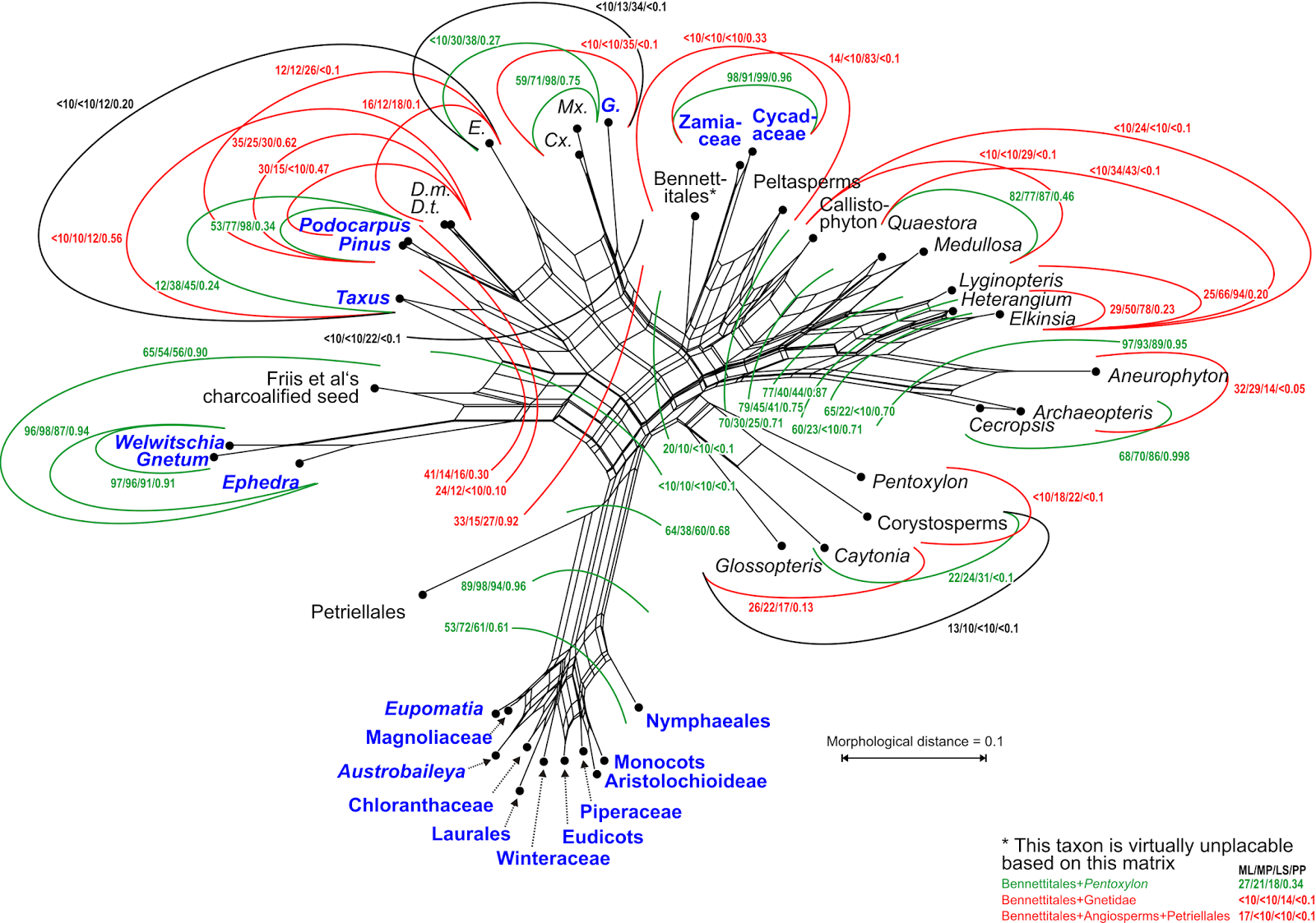
The support patterns indicate that some of the characters are compatible with the tree, but many others are not. Of the 34 internodes (branches) in the shown tree (their fig. 28 shows a strict consensus tree based on a collection of equally parsimonious trees), 12 have lower bootstrap support under parsimony than their competing alternatives (Fig. 1). Support may be generally low for any alternative, but the ones in the tree can be among the worst.

The main problem is that the matrix simply does not provide enough tree-like signal to infer a tree. Delta Values (Holland et al. 2002) can be used as a quick estimate for the treelikeliness of signal in a matrix. In the case of large all-spermatophyte matrices (Hilton & Bateman 2006; Friis et al. 2007; Rothwell, Crepet & Stockey 2009; Crepet & Stevenson 2010), the matrix Delta Values (mDV) are ≥ 0.3. For comparison, molecular matrices resulting in more or less resolved trees have mDV of ≤ 0.15. The individual Delta Values (iDV), which can be an indicator of how well a taxon behaves during tree inference, go down to 0.25 for extant angiosperms – very distinct from all other taxa in the all-spermatophyte matrices with low proportions of missing data/gaps – and reach values of 0.35 for fossil taxa with long-debated affinities.

The newest 2016 matrix is no exception with a mDV of 0.322 (the highest of all mentioned matrices), and iDVs range between 0.26 (monocots and other extant angiosperms) and 0.39 for Doylea mongolica (a fossil with very few scored characters). In the original tree, Doylea (represented by two taxa) is part of the large grade and indicated as the sister to Gnetidae (or Gnetales) + angiosperms (molecular trees associate the Gnetidae with conifers and Ginkgo). According to the bootstrap analysis, Doylea is closest to the extant Pinales, the modern conifers. Coiro et al. found the same using Bayesian inference. Their posterior probability (PP) of a Doylea-Podocarpus-Pinus clade is 0.54, and Rothwell & Stockey’s Doylea-Ginkgo-angiosperm clade conflicts with a series of splits with PPs up to 0.95.

Figure 1. Parsimony bootstrap network based on 10,000 pseudoreplicate trees
inferred from the matrix of Rothwell & Stockey.
Edges not found in the authors’ tree in red, edges also found in the tree in green.
Extant taxa in blue bold font. The edge length is proportional to the frequency of the
according split (taxon bipartition, branch in a possible tree) in the pseudoreplicate
tree sample. The network includes all edges of the authors’ tree except for
Doylea + Gnetidae + Petriellales + angiosperms vs. all other gymnosperms and
extinct seed plant groups. Such a split has also no bootstrap support (BS < 10)
using least-square and maximum likelihood optimum criteria.

Do the data require a tree?

As David made a point in an earlier post, neighbour-nets are not really “phylogenetic networks” in the evolutionary sense. Being unrooted and 2-dimensional, they don’t depict a phylogeny, which has to be a sort of (rooted) tree, a one-dimensional graph with time as the only axis (this includes reticulation networks where nodes can be the crossing point of two internodes rather than their divergence point). The neighbour-net algorithm is an extension into two dimensions of the neighbour-joining algorithm, the latter infers a phylogenetic tree serving a distance criterion such as minimum evolution or least-squares (Felsenstein 2004). Essentially, the neighbour-net is a ‘meta-phylogenetic’ graph inferring and depicting the best and second-best alternative for each relationship. Thus, neighbour-nets can help to establish whether the signal from a matrix, treelike or not as it is the cases here, supports potential and phylogenetic relationships, and explore the alternatives much more comprehensively than would be possible with a strict-consensus or other tree (Fig. 2).

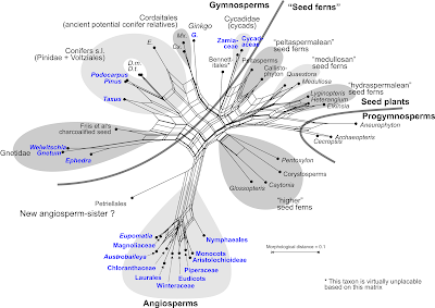
Figure 2. Neighbour-net based on a mean distance matrix inferred
from the matrix of Rothwell & Stockey.
The distance to the "progymnosperms", a potential ancestral group of the
seed plants, can be taken as a measurement for the derivedness of each
major group. The primitive seed ferns are placed between progymnosperms
 and the gymnosperms connected by partly compatible edge bundles; the
putatively derived "higher seed ferns" isolated between the progymnosperms
and the long-edged angiosperms. Shared edge-bundles and 'neighbourness'
reflect quite well potential phylogenetic relationships and eventual ambiguities,
as in the case of Gnetidae. Colouring as in Figure 1; some taxon names
are abbreviated.

In addition, neighbour-nets usually are better backgrounds to map patterns of conflicting or partly conflicting support seen in a bootstrap, jackknife or Bayesian-inferred tree sample. In Fig. 3, I have mapped the bootstrap support for alternative taxon bipartitions (branches in a tree) on the background of the neighbour-net in Fig. 2.

Obvious and less-obvious relationships are simultaneously revealed, and their competing support patterns depicted. Based on the graph, we can see (edge lengths of the neighbour-net) that there is a relatively weak primary but substantial bootstrap support for the Petriellales (a recently described taxon new to the matrix) as sister to the angiosperms. Several taxa, or groups of closely related taxa, are characterised by long terminal edges/edge bundles, rooting in the boxy central part of the graph. Any alternative relationship of these taxa/taxon groups receives equally low support, but there are notable differences in the actual values.

There is little signal to place most of the fossil “seed ferns” (extinct seed plants) in relation to the modern groups, and a very ambiguous signal regarding the relationship of the Gnetidae (or Gnetales) with the two main groups of extant seed plants, the conifers (Pinidae; see C. Earle’s gymnosperm database) and angiosperms (for a list and trees, see P. Stevens’ Angiosperm Phylogeny Website).

The Gnetidae is a strongly distinct (also genetically) group of three surviving genera, being a persistent source of headaches for plant phylogeneticists. Placed as sister to the Pinaceae (‘Gnepine’ hypothesis) in early molecular trees (long-branch attraction artefact), the currently favoured hypothesis (‘Gnetifer’) places the Gnetidae as sister to all conifers (Pinatidae) in an all-gymnosperm clade (including Gingko and possibly the cycads).

As favoured by the branch support analyses, and contrasting with the preferred 2016 tree, the two Doyleas are placed closest to the conifers, nested within a commonly found group including the modern and ancient conifers and their long-extinct relatives (Cordaitales), and possibly Ginkgo (Ginkgoidae). In the original parsimony strict consensus tree, they are placed in the distal part as sister to a Gnetidae and Petriellales + angiosperms (possibly long-branch attraction). The grade including the ‘primitive seed ferns’ (Elkinsia through Callistophyton), seen also in Rothwell and Stockey’s 2016 tree, may be poorly supported under maximum parsimony (the criterion used to generate the tree), but receives quite high support when using a probabilistic approach such as maximum likelihood bootstrapping or Bayesian inference to some degree (Fig. 3; Coiro, Chomicki & Doyle 2017).

Figure 3. Neighbour-net from above used to map alternative support patterns.
Numbers refer to non-parametric bootstrap (BS) support for alternative phylogenetic
splits under three optimality criteria: maximum likelihood (ML) as implemented in
RAxML (using MK+G model), maximum parsimony (MP), and least-squares
(via neighbour-joining, NJ; using PAUP*); and Bayesian posterior probabilties
(using MrBayes 3.2; see Denk & Grimm 2009, for analysis set-up). The circular
arrangement of the taxa allows tracking most edges in the authors’ tree and their,
sometimes better supported, alternatives. The edge lengths provide direct
information about the distinctness of the included taxa to each other; the structure
of the graph informs about the how tree-like the signal is regarding possible
phylogenetic relationships or their alternatives. Colouring as in Figure 1;
some taxon names are abbreviated.

Numerous morphological matrices provide non-treelike signals. A tree can be inferred, but its topology may be only one of many possible trees. In the framework of total evidence, this may be not such a big problem, because the molecular partitions will predefine a tree, and fossils will simply be placed in that tree based on their character suites. Without such data, any tree may be biased and a poor reflection of the differentiation patterns.

By not forcing the data in a series of dichotomies, neighbour-nets provide a quick, simple alternative. Unambiguous, well-supported branches in a tree will usually result in tree-like portions of the neighbour net. Boxy portions in the neighbour-net pinpoint the ambiguous or even problematic signals from the matrix. Based on the graph, one can extract the alternatives worth testing or exploring. Support for the alternatives can be established using traditional branch support measures. Since any morphological matrix will combine those characters that are in line with the phylogeny as well as those that are at odds with it (convergences, character misinterpretations), the focus cannot be to infer a tree, but to establish the alternative scenarios and the support for them in the data matrix.

References

Coiro M, Chomicki G, Doyle JA. 2017. Experimental signal dissection and method sensitivity analyses reaffirm the potential of fossils and morphology in the resolution of seed plant phylogeny. bioRxiv DOI:10.1101/134262

Crepet WL, Stevenson DM. 2010. The Bennettitales (Cycadeoidales): a preliminary perspective of this arguably enigmatic group. In: Gee CT, ed. Plants in Mesozoic Time: Morphological Innovations, Phylogeny, Ecosystems. Bloomington: Indiana University Press, pp. 215-244.

Denk T, Grimm GW. 2009. The biogeographic history of beech trees. Review of Palaeobotany and Palynology 158: 83-100.

Felsenstein J. 2004. Inferring Phylogenies. Sunderland, MA, U.S.A.: Sinauer Associates Inc.

Friis EM, Crane PR, Pedersen KR, Bengtson S, Donoghue PCJ, Grimm GW, Stampanoni M. 2007. Phase-contrast X-ray microtomography links Cretaceous seeds with Gnetales and Bennettitales. Nature 450: 549-552 [all important information needed for this post is in the supplement to the paper; a figure showing the actual full analysis results can be found at figshare]

Hilton J, Bateman RM. 2006. Pteridosperms are the backbone of seed-plant phylogeny. Journal of the Torrey Botanical Society 133: 119-168.

Holland BR, Huber KT, Dress A, Moulton V. 2002. Delta Plots: A tool for analyzing phylogenetic distance data. Molecular Biology and Evolution 19: 2051-2059.

Rothwell GW, Crepet WL, Stockey RA. 2009. Is the anthophyte hypothesis alive and well? New evidence from the reproductive structures of Bennettitales. American Journal of Botany 96: 296–322.

Rothwell GW, Nixon K. 2006. How does the inclusion of fossil data change our conclusions about the phylogenetic history of the euphyllophytes? International Journal of Plant Sciences 167: 737–749.

Rothwell GW, Stockey RA. 2016. Phylogenetic diversification of Early Cretaceous seed plants: The compound seed cone of Doylea tetrahedrasperma. American Journal of Botany 103: 923–937.

Schliep K, Potts AJ, Morrison DA, Grimm GW. 2017. Intertwining phylogenetic trees and networks. Methods in Ecology and Evolution DOI:10.1111/2041-210X.12760.

Connecting tree and network edges


I have struggled over the years to try to understand the relationship between trees and networks. In one sense, networks are generalizations of trees, and in another sense a tree is just a simplified network. But it is not always that simple.

For example, not all networks can be created by adding edges to a tree (see Networks vs augmented trees); so the connection between trees and networks is not always obvious. Moreover, it is not always easy to determine which tree edges are present in any given network, or which network edges are present in a given tree.

Nevertheless, this should be basic information in phylogenetics — otherwise, how can we know when a tree is adequate for our purposes, or when a network is needed?

It turns out that I have not been alone in struggling to connect trees and networks. Fortunately, some of these other people decided to actually do something about it, rather than simply struggling on. As a result, a computerized way to relate much of the important information connecting trees with networks now exists.
Klaus Schliep, Alastair J. Potts, David A. Morrison and Guido W. Grimm
Intertwining phylogenetic trees and networks.
Methods in Ecology and Evolution (Early View)
To quote the authors:
Here we provide a framework, implemented in the PHANGORN library in R, to transfer information between trees and networks. This includes: (i) identifying and labelling equivalent tree branches and network edges, (ii) transferring tree branch-support to network edges, and (iii) mapping bipartition support from a sample of trees (e.g. from bootstrapping or Bayesian inference) onto network edges.
These three functions are illustrated in this figure, taken from the paper. It should be self-explanatory to anyone who has tried to relate the edges of trees and networks; but if it is not, then you can read an explanation in the paper.


The R library referred to, including the source code, along with some examples and vignettes, can be accessed on the PHANGORN CRAN page.

Note that PHANGORN (originally created by Klaus Schliep) also contains other functions related to estimating phylogenetic trees and networks, using maximum likelihood, maximum parsimony, distance methods and hadamard conjugation. Specifically, it allows you to: estimate phylogenies, compare trees and models, and explore tree space and visualize phylogenetic trees and split graphs.

James Bond, alcoholic


Merry Christmas to everyone. As usual for this blog at this time of year, for your Christmas reading we will take a look at a particular aspect of human consumption, in this case alcohol.

James Bond was created in 1953 by Ian Fleming (who also created Chitty-Chitty-Bang-Bang, The Magical Car), and over a 14-year period there was a series of 12 novels and two short-story collections. The rights to the character were purchased for the film world in the 1960s, so that over the past 50 years we have had a franchise of 24 official films, plus two other licensed ones (Casino Royale in 1967, and Never Say Never Again in 1983).

Actually, the first licensed Bond film was a long-forgotten one made for CBS TV in 1954. This was a 1-hour version of Casino Royale, starring Barry Nelson as Bond, Peter Lorre as Le Chiffre, and Linda Christian as a renamed Vesper Lynd (see Barry Nelson - den bortglömde Bond).

This movie infographic (excluding the 2015 film, and the unofficial films) is from The Economist.


The Bond character

James Bond has been portrayed in films officially by six different actors, but the character remains essentially the same, although somewhat different from the one depicted in the books.

In early 1997, the monthly magazine Men's Health published an article in which doctors and psychologists commented on the life and lifestyle of the Bond character, the world's most un-secret secret agent (see Sprit, kvinnor och cigarretter tog livet av James Bond). The results were not good — Bond was either dead or close to it, as he was a paranoid, impotent alcoholic.

Bond's psychological profile was that of an emotionally stunted psychopath of type A who suffers from post-traumatic stress. According to Fleming's books, Bond was orphaned at age 11 (his parents died in a mountaineering accident), he lost his virginity in a brothel in Paris at 16, and killed his first mistress the following year. An ideal man to be a licensed assassin.

His massive daily alcohol consumption (all carefully documented in both the books and films) makes him a category 3 alcoholic. This means that he couldn't possibly have done his actual job competently; and it should also have led to violent temper outbursts (which may explain the government-sanctioned killing sprees). The liquor should also have led to a shrinking of his genitals, and have damaged his liver to the extent that it could no longer break down estrogen, so that he started to develop breasts and become impotent. His well-documented sexual excesses would also make him a prime candidate for sexually transmitted diseases. On top of this, the books (but not the films) also document a comprehensive smoking habit.

Bond was, of course, a form of wish-fulfillment for his creator, Ian Fleming, who was also a heavy drinker and smoker. He died of a heart attack at age 56, an age that Bond himself could not possibly have out-lived. Bond was more in danger from his own lifestyle than from SMERSH, or anyone else bent on world domination.

Bond is thus more a collection of memes than an actual character. This infographic is from the GBShowPlates website, and summarizes Bond's lifestyle.


The Bond drinks

Just about every aspect of Bond's career has been analyzed, and ranked, from the music to the cars to the watches, and most especially the women (the so-called "Bond girls"). However, much of the interest seems to lie in the booze, which is what we will look at here.

Along with coffee (and, once, tea), Bond has consumed copious amounts of alcohol, which he tends to drink alone, or in private settings. He is also what is known as a "label drinker", in that the brand is at least as important as the bottle's contents. This is a gift for the liquor industry, who, along with the car industry, are perpetually looking for opportunities for "brand placement" in films and sporting events. Fleming was chastised for introducing this into his books, but he simply replied that it was an attempt to round-out the character.

As far as the novels are concerned, they have received special medical attention by Graham Johnson, Indra Neil Guha, Patrick Davies (2013. Were James Bond’s drinks shaken because of alcohol induced tremor? British Medical Journal 347: f7255). They recorded every drink consumed in every book, calculated the number of alcohol units involved, and then converted that to daily intake (since the books are quite clear about their time span).

Their results are summarized in this infographic, from their article.


Basically, the medical results were as before:
Across 12 of the 14 books, 123.5 days were described, though Bond was unable to consume alcohol for 36 days because of external pressures (admission to hospital, incarceration, rehabilitation). During this time he was documented as consuming 1150.15 units of alcohol. Taking into account days when he was unable to drink, his average alcohol consumption was 92 units a week (1150 units over 87.5 days). Inclusion of the days incarcerated brings his consumption down to 65.2 units a week. His maximum daily consumption was 49.8 units (From Russia with Love day 3). He had 12.5 alcohol free days out of the 87.5 days on which he was able to drink.
Furthermore, when we plotted Bond's alcohol consumption over time, his intake dropped in the middle of his career but gradually increased towards the end. This consistent but variable lifetime drinking pattern has been reported in patients with alcoholic liver disease.
UK NHS [National Health Service] recommendations for alcohol consumption state that an adult male should drink no more than 21 units a week, with no more than 4 units on any one day, and at least two alcohol free days a week. James Bond's drinking habits are well in excess of each of these three parameters. This level of consumption makes him a category 3 drinker (>60 g alcohol / day) and therefore in the highest risk group for malignancies, depression, hypertension, and cirrhosis. He is also at high risk of suffering from sexual dysfunction, which would considerably affect his womanising.
Analyzing the films is more difficult. A number of people have tackled this task, including Nerdist, The Grocer, and Atomic Martinis (now defunct, but repeated on the website of the world's only James Bond Museum, in Sweden), and David Leigh. The basic problem seems to be whether the alcohol is "spotted either in hand, glass or in the background". Also, "The major problem is 007’s frequent enjoyment of multiple bottles of champagne, or portions of bottles of liquor ... it is often impossible to determine exactly how many separate drinks came from a given bottle."

The following infographic (not including the 2015 movie or the unofficial films) is derived from one produced at Buddy Loans. However, some of the people at Reddit were not happy with the original, so it was redesigned, as shown here.


The people at Nerdist took the data from this film infographic, converted it from units of alcohol to grams of alcohol, and then used this to estimate Bond’s total alcohol content. This yields a Blood Alcohol Content of 3.7%. "While some humans have survived a BAC of past 1%, it generally holds that anything past 0.5% will either kill you or leave you seriously poisoned. Therefore ... Bond’s tipsy tally is enough to put a man past a safe limit seven times over."

At The Grocer, they have also pointed out the relative booziness of the various Bond incarnations, by calculating the average intake per film by each actor, in units of alcohol:
Sean Connery
George Lazenby
Roger Moore
Timothy Dalton
Pierce Brosnan
Daniel Craig
11
  9
11
  4.5
12
20
Finally, we need a phylogenetic network, of course. I collated the presence/absence of each drink type for each book and movie (excluding the 2015 film) from the book by David Leigh (2012. The Complete Guide to the Drinks of James Bond, 2nd edition. Kindle), and then updated this where it clearly disagrees with other sources. (For example, no mention is made of sherry, and yet it is involved in one of the most popular Bond scenes from the film version of Diamonds are Forever.) I then analyzed the data using a NeighborNet. (James Bond Memes has tried an ordination analysis of the same data source.)


The books are shown in red, and the early films starring Connery and Lazenby are shown in blue (including Connery's later Never Say Never Again). These books and films are almost all at the top and right of the network, indicating that they have a distinct collection of drink types compared to the later films. I suspect that this reflects increasing use of "product placements" in the films. The only book plus movie combination that has similar drinks is You Only Live Twice. Interestingly, the Skyfall movie (from 2012) seems to return to the drinks genre of the earlier works, even though the alcohol consumption is much higher. The most unusual works were the Goldfinger and On Her Majesty's Secret Service books, where a number of drink styles were consumed that appeared nowhere else in the canon.

As noted by Johnson et al. (quoted above):
Despite his alcohol consumption, [Bond] is still described as being able to carry out highly complicated tasks and function at an extraordinarily high level. This is likely to be pure fiction.

Why are splits graphs still called phylogenetic networks?


This is an issue that has long concerned me, and which I think causes a lot of confusion among biologists. A phylogenetic tree is usually a clear concept — to a biologist, it is a diagram that displays a hypothesis of evolutionary history. The expectation, then, is that a phylogenetic network does the same thing for reticulate evolutionary histories. However, this is not true of splits graphs; and so there is potential confusion.

Mathematically, of course, a phylogenetic tree is a directed acyclic line graph. It is usually constructed, in practice, by first producing an undirected graph based on some pattern-analysis procedure, and then nominating one of the nodes or edges as the root (say, by specifying an outgroup). So, the mathematics is not really connected to the biological interpretation. To a mathematician, the tree is a set of nodes connected by directed edges, and the nodes could represent anything at all, as could the edges. It is the biologist who artificially imposes the idea that the nodes represent real historical organisms connected by the flow of evolution — ancestors connected to descendants by evolutionary events.

A phylogenetic network should logically be a generalization of this idea of a phylogenetic tree, adding the possibility of evolutionary relationships due to gene flow, in addition to the ancestor-descendant relationships. This can be done, but it is only partly done by splits graphs.

That is, a splits graph generalizes the idea of an undirected line graph (an unrooted tree), but not a directed acyclic graph (a rooted tree). It follows the same logic of using a pattern-analysis procedure to produce an undirected graph, although the graph can have reticulations, and thus is a network rather than necessarily being a bifurcating tree. However, it is not straightforward to specify a root in a way that will turn this into an acyclic graph. So, in general it does not represent a phylogeny.

Indeed, splits graphs are simply one form of multivariate pattern analysis, along with clustering and ordination techniques, which are familiar as data-display methods in phenetics (see Morrison D.A. 2014. Phylogenetic networks — a new form of multivariate data summary for data mining and exploratory data analysis. Wiley Interdisciplinary Reviews: Data Mining and Knowledge Discovery 4: 296-312). In this sense, it makes no difference whatsoever what the data represent — they can be data used for phylogenetics, or they could be any other form of multivariate data. Indeed, this point is illustrated in many of the posts in this blog, which can be accessed in the Analyses page.

So, unlike unrooted trees, unrooted splits graphs are not a route to producing a phylogenetic diagram. Mind you, they are a very useful form of multivariate data analysis in their own right, and I value them highly as a form of exploratory data analysis. But that doesn't make them phylogenetic networks in the biological sense.

So, isn't it about time we stopped calling splits graphs "phylogenetic networks"? They aren't, to a biologist, so why call them that?

Walking can be more dangerous than cycling


We are often told that flying is the safest way to travel, at least as far as the use of commercial airlines is concerned. In an early stand-up comedy routine, Shelley Berman noted: "Statistics prove that flying is the safest way to travel. I don't know how much consideration they've given to walking!" Well, actually, they have included walking.

Governments like to keep a track of these things, and the Department for Transport in Great Britain has released statistics on "Passenger casualty rates for different modes of travel" for 2003-2012. These modes include:
  • Air (passenger casualties in accidents involving UK registered airline aircraft)
  • Rail (passenger casualties involved in train accidents and accidents occurring through movement of railway vehicles)
  • Water (passenger casualties on UK registered merchant vessels)
  • Bus or coach (passenger casualties)
  • Car (driver and passenger casualties)
  • Van (driver and passenger casualties)
  • Motorcycle (driver and passenger casualties)
  • Pedal cycle
  • Pedestrian
The data are yearly averages for Great Britain from 2003-2012 inclusive, standardized as persons per billion passenger kilometres. The data are provided separately for the number of people killed, seriously injured, or slightly injured.

As usual, we can employ a phylogenetic network as a form of exploratory data analysis for these data. I first used the manhattan distance to calculate the similarity of the seven transportation modes for which there are complete data, followed by a Neighbor-net analysis to display the between-mode similarities as a phylogenetic network. So, modes that are closely connected in the network are similar to each other based on their accident figures across the ten years, and those that are further apart are progressively more different from each other.


The probability of incidents increases from right to left in the graph.

Some notable conclusions from the data are:
  • The probabilities of being killed, seriously injured or even slightly injured are all minuscule for air travel compared to anything else. This is a topic explored more thoroughly in an earlier blog post (A network analysis of airplane disasters).
  • You are much more likely to be injured in a bus than in a truck, but more likely to be killed in the truck than in the bus.
  • You are slightly more likely to be killed walking than cycling, but much more likely to be injured cycling.
  • A motorbike is the most effective way to get killed or seriously injured in Britain.

The walking versus cycling data are likely to surprise many people, but the average data across the 10 years are clear:

Pedestrian
Pedal cycle
Motorcycle
Killed
31
27
92
Seriously injured
328
550
1,043
Slightly injured
1,245
3,190
2,997

Danny Yee (Walking and cycling: relative risks) provides one explanation:
People who wouldn't even contemplate wearing special high-visability clothing or a helmet for a walk to the shops do so when cycling the same route.

A limitation of turning splits graphs into reticulate networks


Splits graphs are a useful way of displaying contradictory information within evolutionary datasets, either incompatible characters (ie. those that cannot fit onto a single tree) or incompatible trees. Since the graphs are unrooted, they are usually treated as a form of multivariate data display, rather than interpreted as depicting evolutionary history.

However, it is possible to turn a splits graph into a evolutionary network (sometimes called a reticulation network) once a root is specified (Huson and Klöpper 2007). This is true irrespective of whether the splits are derived from character data (Huson and Kloepper 2005), in which case it usually called a recombination network, or whether they come from a set of trees (Huson et al. 2005), in which case it is usually called a hybridization network.

The SplitsTree4 program (Huson and Bryant 2006) carries out the relevant calculations under algorithms entitled Reticulation Network, Recombination Network or Hybridization Network, although these all produce the same outcome once the set of splits has been determined. These options are no longer available from the menu system (in the current release of the program), but they can still be effected via the Configure Pipeline menu option.

The point of this post is to point out that the calculations are affected by the same limitation that has been pointed out before under other circumstances (see the post A fundamental limitation of hybridization networks?). That is, reticulation cycles with three or fewer outgoing arcs are not uniquely defined with respect to rooted splits — there are three equally optimal mathematical solutions. In practice, this means that in a situation where two taxa are involved in producing a third taxon we cannot decide from the splits alone which is the reticulate taxon and which are the two "parents" (eg. which one is the hybrid).

An example

I will illustrate this point with a simple example. The data are taken from Wendel et al. (1991). The data consist of the presence-absence of 76 nuclear allozyme loci and 13 nuclear restriction sites, for five plant taxa, one of which is the outgroup. The first graph shows the splits graph using the default options in SplitsTree4 — both the NeighborNet and the ParsimonySplits analyses produce the same graph, which identifies a single reticulation.


In SplitsTree4, the outgroup for rooting the splits graph must be the first taxon in the datafile, which in this case is Gossypium robinsonii. The following three graphs are the result of then choosing the ReticulateNetwork analysis. They differ by having, respectively, Gossypium bickii as the final taxon in the dataset, Gossypium sturtianum as the final taxon, and Gossypium australe + Gossypium nelsonii as the final two taxa. Note that the ReticulateNetwork algorithm always identifies the dataset's final taxon as the reticulate one.


So, the hybrid taxon is indeterminable from the data given, and the algorithm simply makes a (consistent) choice from among the three possibilities. [That is, the algorithm chooses as the reticulate arc whichever of the three outgoing arcs is latest in the dataset.]

The original authors suggest that the nuclear and other data "indicate a biphyletic ancestry of G. bickii. Our preferred hypothesis involves an ancient hybridization, in which G. sturtianum, or a similar species, served as the maternal parent with a paternal donor from the lineage leading to G. australe and G. nelsoni." This doesn't quite match any of the three rooted networks shown above.

References

Huson DH, Bryant D (2006) Application of phylogenetic networks in evolutionary studies. Molecular Biology and Evolution 23: 254-267.

Huson DH, Kloepper TH (2005) Computing recombination networks from binary sequences. Bioinformatics 21: ii159-ii165.

Huson DH, Klöpper TH (2007) Beyond galled trees – decomposition and computation of galled networks. Lecture Notes in Bioinformatics 4453: 211-225.

Huson DH, Klöpper T, Lockhart PJ, Steel MA (2005) Reconstruction of reticulate networks from gene trees. Lecture Notes in Bioinformatics 3500: 233-249.

Wendel JF, Stewart JM, Rettig JH (1991) Molecular evidence for homoploid reticulate evolution among Australian species of Gossypium. Evolution 45: 694-711.

A phylogenetic network of late-night US television shows


"Late night" broadcasting on United States network / cable TV starts at about 11:00 or 11:30 pm, and goes for a couple of hours. Many networks broadcast similar shows during this time, which directly compete against each other for the available audience (which is currently estimated to be slightly in excess of 10 million people per night at 11:30 pm). Many of these shows have been on for a long time. Most of them are recorded on several weekday nights in front of a live audience, and they are usually associated with only a very few presenters over time (almost always men!).


For example, since the early 1990s we have had:
NBC Tonight Show


NBC Late Night


CBS Late Show
CBS Late Late Show


ABC Kimmel Live
ABC Nightline

ComedyCentral Daily Show

ComedyCentral Colbert Report
TBS Conan
11:35-12:35


12:35-01:35


11:35-12:35
12:35-01:35


11:35-12:35
12:35-01:05

11:00-11:30

11:30-12:00
11:00-12:00
Jay Leno 1992-2009
Conan O'Brien 2009-2010
Jay Leno 2010-2014
Jimmy Fallon 2014-
David Letterman 1982-1993
Conan O'Brien 1993-2009
Jimmy Fallon 2009-2014
Seth Meyers 2014-
David Letterman 1993-2015
Tom Snyder 1995-1999
Craig Kilborn 1999-2004
Craig Ferguson 2005-2014
James Corden 2015-
Jimmy Kimmel 2003-
Ted Koppel 1980-2005
Three-anchor team 2005-
Craig Kilborn 1996-1998
Jon Stewart 1999-
Stephen Colbert 2005-2014
Conan O'Brien 2010-

Eventually, the presenters retire or move elsewhere, and the other presenters then move around among the shows. This has lead to the so-called "Late night wars", in which the NBC studio executives in charge repeatedly show that their personnel management skills are often lacking. For example, David Letterman was expected to replace Johnny Carson when he retired as the host of the NBC Tonight Show in 1992, but the job was given to Jay Leno, instead. So, Letterman moved to a directly competing show on CBS. When Leno subsequently moved to another show, Conan O'Brien took over. However, Leno then moved back again, and so O'Brien moved to a directly competing show on TBS. The media interest in these shenanigans exceeded their interest in the shows themselves.

Another substantial decision was that by ABC, at the end of 2012, to swap the timelsots of Nightline (which used to run 11:35-12:00) and Kimmel Live (which ran 12:00-13:00). This had a notable effect on the audience numbers, because Nightline was one of the top two shows in its original timeslot whereas Kimmel Live currently gets about 1 million viewers fewer per night in that same slot. On the other hand Nightline in its new timelsot gets about the same audience as Kimmel Live did when it occupied the slot. That seems to be a net loss of audience for ABC.

The Nielsen Media Research viewing data are available online at the TV by the Numbers site. They provide the weekly averages for each show in millions of viewers, based on what is known as "live plus same day" viewing (ie. the audience at the time of broadcast plus same-day viewing of video recordings). The data I have looked at run from early December 2011 to the end of December 2014 (161 weeks). Unfortunately, these data rely on NBC press releases (rather than direct access to Nielsen), so there are some missing data.

The comparison of these shows can be visualized using a phylogenetic network, as a tool for exploratory data analysis. To create the network, I first calculated the similarity of the nine shows using the manhattan distance; and a Neighbor-net analysis was then used to display the between-show similarities as a phylogenetic network. So, shows that are closely connected in the network are similar to each other based on their audience figures across the three years, and those that are further apart are progressively more different from each other.


The network shows a gradient of increasing audience size, from bottom-left to top-right. So, the Tonight Show consistently got a average nightly audience of c. 3.5 million people, while Conan had c. 0.8 million. The two CBS shows both consistently did somewhat worse than their NBC timeslot competitors.

The two ABC shows apparently did well, but this is confounded by the timeslot swap noted above. Nightline did well for the first year (before it was moved) but not for the second two years, while Kimmel Live did the opposite. This is what creates the big reticulation in the middle of the network, as all of the other shows had fairly consistent audiences throughout the three years.

However, there was a steady decrease in the total audience size across the three years, from c. 12 million per night (at 11:30 pm) at the end of 2011 to c. 10 million at the end of 2014. The only major exception to this was at the time when Jimmy Fallon took over from Jay Leno (early 2014). For several weeks the Tonight Show audience increased to >8 million per night, so that the total audience was c. 15.5 million (a 50% increase). This shows just how many people are available to be added to the late-night viewing, compared to how many watch regularly. So, why are they not watching in the other weeks? It seems that Late Night Television is not reaching its full potential.