26Feb / 2018

Tossing coins: linguistic phylogenies and extensive synonymy

The procedures by which linguists sample data when carrying out phylogenetic analyses of languages are sometimes fundamentally different from the methods applied in biology. This is particularly obvious in the matter of the sampling of data for analysis, which I will discuss in this post.

Sampling data in historical linguistics

The reason for the difference is straightforward: while biologists can now sample whole genomes and search across those genomes for shared word families, linguists cannot sample the whole lexicon of several languages. The problem is not that we could not apply cognate detection methods to whole dictionaries. In fact there are recent attempts that try to do exactly this (Arnaud et al. 2017). The problem is that we simply do not know exactly how many words we can find in any given language.

For example, the Duden, a large lexicon of the German language, for example, recently added 5000 more words, mostly due to recent technological innovations, which then lead to new words which we frequently use in German, such as twittern "to tweet", Tablet "tablet computer", or Drohnenangriff "drone attack". In total, it now lists 145,000 words, and the majority of these words has been coined in complex processes involving language-internal derivation of new word forms, but also by a large amount of borrowing, as one can see from the three examples.

One could argue that we should only sample those words which most of the speakers in a given language know, but even there we are far from being able to provide reliable statistics, not to speak of the fact that it is also possible that these numbers vary greatly across different language families and cultural and sociolinguistic backgrounds. Brysbaert et al. (2016), for example, estimate that

an average 20-year-old native speaker of American English knows 42,000 lemmas and 4,200 non-transparent multiword expressions, derived from 11,100 word families.

But in order to count as "near-native" in a certain language, including the ability to pursue studies at a university, the Common European Framework of Reference for Languages, requires only between 4000 and 5000 words (Milton 2010, see also List et al. 2016). How many word families this includes is not clear, and may, again, depend directly on the target language.

Lexicostatistics

When Morris Swadesh (1909-1967) established the discipline of lexicostatistics, which represented the first attempt to approach the problems we face in historical linguistics with the help of quantitative methods. He started from a sample of 215 concepts (Swadesh 1950), which he later reduced to only 100 (Swadesh 1955), because he was afraid that some concepts would often be denoted by words that are borrowed, or that would simply not be expressed by single words in certain language families. Since then, linguists have been trying to refine this list further, either by modifying it (Starostin 1991 added 10 more concepts to Swadesh's list of 100 concepts), or by reducing it even further (Holman et al. 2008 reduced the list to 40 concepts).

While it is not essential how many concepts we use in the end, it is important to understand that we do not start simply by comparing words in our current phylogenetic approaches, but instead we sample parts of the lexicon of our languages with the help of a list of comparative concepts (Haspelmath 2010), which we then consecutively translate into the target languages. This sampling procedure was not necessarily invented by Morris Swadesh, but he was first to establish its broader use, and we have directly inherited this procedure of sampling when applying our phylogenetic methods (see this earlier post for details on lexicostatistics).

Synonymy in linguistic datasets

Having inherited the procedure, we have also inherited its problems, and, unfortunately, there are many problems involved with this sampling procedure. Not only do we have difficulties determining a universal diagnostic test list that could be applied to all languages, we also have considerable problems in standardizing the procedure of translating a comparative concept into the target languages, especially when the concepts are only loosely defined. The concept "to kill", for example, seems to be a rather straightforward example at first sight. In German, however, we have two words that could express this meaning equally well: töten (cognate with English dead) and umbringen (partially cognate with English to bring). In fact, as with all languages in the world, there are many more words for "to kill" in German, but these can easily be filtered out, as they usually are euphemisms, such as eliminieren "to eliminate", or neutralisieren "to neutralize". The words töten and umbringen, however, are extremely difficult to distinguish with respect to their meaning, and speakers often use them interchangeably, depending, perhaps, on register (töten being more formal). But even for me as a native speaker of German, it is incredibly difficult to tell when I use which word.

One solution to making a decision as to which of the words is more basic could be corpus studies. By counting how often and in which situations one term is used in a large corpus of German speech, we might be able to determine which of the two words comes closer to the concept "to kill" (see Starostin 2013 for a very elegant example for the problem of words for "dog" in Chinese). But in most cases where we compile lists of languages, we do not have the necessary corpora.

Furthermore, since corpus studies on competing forms for a given concept are extremely rare in linguistics, we cannot exclude the possibility that the frequency of two words expressing the same concept is in the end the same, and the words just represent a state of equilibrium in which speakers use them interchangeably. Whether we like it or not, we have to accept that there is no general principle to avoid these cases of synymony when compiling our datasets for phylogenetic analyses.

Tossing coins

What should linguists do in such a situation, when they are about to compile the dataset that they want to analyze with the modern phylogenetic methods, in order to reconstruct some eye-catching phylogenetic trees? In the early days of lexicostatistics, scholars recommended being very strict, demanding that only one word in a given language should represent one comparative concept. In cases like German töten and umbringen, they recommended to toss a coin (Gudschinsky 1956), in order to guarantee that the procedure was as objective as possible.

Later on, scholars relaxed the criteria, and just accepted that in a few — hopefully very few — cases there would be more than one word representing a comparative concept in a given language. This principle has not changed with the quantitative turn in historical linguistics. In fact, thanks to the procedure by which cognate sets across concept slots are dichotomized in a second step, scholars who only care for the phylogenetic analyses and not for the real data may easily overlook that the Nexus file from which they try to infer the ancestry of a given language family may list a large amount of synonyms, where the classical scholars simply did not know how to translate one of their diagnostic concepts into the target languages.

Testing the impact of synonymy on phylogenetic reconstruction

The obvious question to ask at this stage is: does this actually matter? Can't we just ignore it and trust that our phylogenetic approaches are sophisticated enough to find the major signals in the data, so that we can just ignore the problem of synonymy in linguistic datasets? In an early study, almost 10 years ago, when I was still a greenhorn in computing, I made an initial study of the problem of extensive synonymy, but it never made it into a publication, since we had to shorten our more general study, of which the synonymy test was only a small part. This study has been online since 2010 (Geisler and List 2010), but is still awaiting publication; and instead of including my quantitative test on the impact of extensive synonymy on phylogenetic reconstruction, we just mentioned the problem briefly.

Given that the problem of extensive synonymy turned up frequently in recent discussions with colleagues working on phylogenetic reconstruction in linguistics, I decided that I should finally close this chapter of my life, and resume the analyses that had been sleeping in my computer for the last 10 years.

The approach is very straightforward. If we want to test whether the choice of translations leaves traces in phylogenetic analyses, we can just take the pioneers of lexicostatistics literally, and conduct a series of coin-tossing experiments. We start from a "normal" dataset that people use in phylogenetic studies. These datasets usually contain a certain amount of synonymy (not extremely many, but it is not surprising to find two, three, or even four translations in the datasets that have been analysed in the recent years). If we now have the computer toss a coin in each situation where only one word should be chosen, we can easily create a large sample of datasets each of which is synonym free. Analysing these datasets and comparing the resulting trees is again straightforward.

I wrote some Python code, based on our LingPy library for computational tasks in historical linguistics (List et al. 2017), and selected four datasets, which are publicly available, for my studies, namely: one Indo-European dataset (Dunn 2012), one Pama-Nyungan dataset (Australian languages, Bowern and Atkinson 2012), one Austronesian dataset (Greenhill et al. 2008), and one Austro-Asiatic dataset (Sidwell 2015). The following table lists some basic information about the number of concepts, languages, and the average synonymy, i.e., the average number of words that a concept expresses in the data.

Dataset	Concepts	Languages	Synonymy
Austro-Asiatic	200	58	1.08
Austronesian	210	45	1.12
Indo-European	208	58	1.16
Pama-Nyungan	183	67	1.1

For each dataset, I made 1000 coin-tossing trials, in which I randomly picked only one word where more than one word would have been given as the translation of a given concept in a given language. I then computed a phylogeny of each newly created dataset with the help of the Neighbor-joining algorithm on the distance matrix of shared cognates (Saitou and Nei 1987). In order to compare the trees, I employed the general Robinson-Foulds distance, as implemented in LingPy by Taraka Rama. Since I did not have time to wait to compare all 1000 trees against each other (as this takes a long time when computing the analyses for four datasets), I randomly sampled 1000 tree pairs. It is, however, easy to repeat the results and compute the distances for all tree pairs exhaustively. The code and the data that I used can be found online at GitHub (github.com/lingpy/toss-a-coin).

Some results

As shown in the following table, where I added the averaged generalized Robinson-Foulds distances for the pairwise tree comparisons, it becomes obvious that — at least for distance-based phylogenetic calculations — the problem of extensive synonymy and choice of translational equivalents has an immediate impact on phylogenetic reconstruction. In fact, the average differences reported here are higher than the ones we find when comparing phylogenetic reconstruction based on automatic pipelines with phylogenetic reconstruction based on manual annotation (Jäger 2013).

Dataset	Concepts	Languages	Synonymy	Average GRF
Austro-Asiatic	200	58	1.08	0.20
Austronesian	210	45	1.12	0.19
Indo-European	208	58	1.16	0.59
Pama-Nyungan	183	67	1.1	0.22

The most impressive example is for the Indo-European dataset, where we have an incredible average distance of 0.59. This result almost seems surreal, and at first I thought that it was my lazy sampling procedure that introduced the bias. But a second trial confirmed the distance (0.62), and when comparing each of the 1000 trial trees with the tree we receive when not excluding the synonyms, the distance
is even slightly higher (0.64).

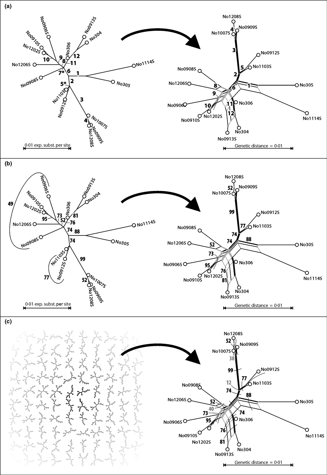
When looking at the consensus network of the 1000 trees (created with SplitsTree4, Huson et al. 2006), using no threshold (to make sure that the full variation could be traced), and the mean for the calculation of the branch lengths, which is shown below, we can see that the variation introduced by the synonyms is indeed real.

The consensus network of the 1000 tree sample for the Indo-European language sample

Notably, the Germanic languages are highly incompatible, followed by Slavic and Romance. In addition, we find quite a lot of variation in the root. Furthermore, when looking the at the table below, which shows the ten languages that have the largest number of synonyms in the Indo-European data, we can see that most of them belong to the highly incompatible Germanic branch.

Language	Subgroup	Synonymous Concepts
OLD_NORSE	Germanic	83
FAROESE	Germanic	77
SWEDISH	Germanic	68
OLD_SWEDISH	Germanic	65
ICELANDIC	Germanic	64
OLD_IRISH	Celtic	61
NORWEGIAN_RIKSMAL	Germanic	54
GUTNISH_LAU	Germanic	50
ORIYA	Indo-Aryan	50
ANCIENT_GREEK	Greek	46

Conclusion

This study should be taken with some due care, as it is a preliminary experiment, and I have only tested it on four datasets, using a rather rough procedure of sampling the distances. It is perfectly possible that Bayesian methods (as they are "traditionally" used for phylogenetic analyses in historical linguistics now) can deal with this problem much better than distance-based approaches. It is also clear that by sampling the trees in a more rigorous manner (eg. by setting a threshold to include only those splits which occur frequently enough), the network will look much more tree like.

However, even if it turns out that the results are exaggerating the situation due to some theoretical or practical errors in my experiment, I think that we can no longer ignore the impact that our data decisions have on the phylogenies we produce. I hope that this preliminary study can eventually lead to some fruitful discussions in our field that may help us to improve our standards of data annotation.

I should also make it clear that this is in part already happening. Our colleagues from Moscow State University (lead by George Starostin in the form of the Global Lexicostatistical Database project) try very hard to improve the procedure by which translational equivalents are selected for the languages they investigate. The same applies to colleagues from our department in Jena who are working on an ambitious database for the Indo-European languages.

In addition to linguists trying to improve the way they sample their data, however, I hope that our computational experts could also begin to take the problem of data sampling in historical linguistics more seriously. A phylogenetic analysis does not start with a Nexus file. Especially in historical linguistics, where we often have very detailed accounts of individual word histories (derived from our qualitative methods), we need to work harder to integrate software solutions and qualitative studies.

References

Arnaud, A., D. Beck, and G. Kondrak (2017) Identifying cognate sets across dictionaries of related languages. In: Proceedings of the 2017 Conference on Empirical Methods in Natural Language Processing 2509-2518.

Bowern, C. and Q. Atkinson (2012) Computational phylogenetics of the internal structure of Pama-Nguyan. Language 88. 817-845.

Brysbaert, M., M. Stevens, P. Mandera, and E. Keuleers (2016) How many words do we know? Practical estimates of vocabulary size dependent on word definition, the degree of language input and the participant’s age. Frontiers in Psychology 7. 1116.

Dunn, M. (ed.) (2012) Indo-European Lexical Cognacy Database (IELex). http://ielex.mpi.nl/.

Geisler, H. and J.-M. List (2010) Beautiful trees on unstable ground: notes on the data problem in lexicostatistics. In: Hettrich, H. (ed.) Die Ausbreitung des Indogermanischen. Thesen aus Sprachwissenschaft, Archäologie und Genetik. Reichert: Wiesbaden.

Greenhill, S., R. Blust, and R. Gray (2008) The Austronesian Basic Vocabulary Database: From bioinformatics to lexomics. Evolutionary Bioinformatics 4. 271-283.

Gudschinsky, S. (1956) The ABC’s of lexicostatistics (glottochronology). Word 12.2. 175-210.

Haspelmath, M. (2010) Comparative concepts and descriptive categories. Language 86.3. 663-687.

Holman, E., S. Wichmann, C. Brown, V. Velupillai, A. Müller, and D. Bakker (2008) Explorations in automated lexicostatistics. Folia Linguistica 20.3. 116-121.

Huson, D. and D. Bryant (2006) Application of phylogenetic networks in evolutionary studies. Molecular Biology and Evolution 23.2. 254-267.

Jäger, G. (2013) Phylogenetic inference from word lists using weighted alignment with empirical determined weights. Language Dynamics and Change 3.2. 245-291.

List, J.-M., J. Pathmanathan, P. Lopez, and E. Bapteste (2016) Unity and disunity in evolutionary sciences: process-based analogies open common research avenues for biology and linguistics. Biology Direct 11.39. 1-17.

List, J.-M., S. Greenhill, and R. Forkel (2017) LingPy. A Python Library For Quantitative Tasks in Historical Linguistics. Software Package. Version 2.6. Max Planck Institute for the Science of Human History: Jena.

Milton, J. (2010) The development of vocabulary breadth across the CEFR levels: a common basis for the elaboration of language syllabuses, curriculum guidelines, examinations, and textbooks across Europe. In: Bartning, I., M. Martin, and I. Vedder (eds.) Communicative Proficiency and Linguistic Development: Intersections Between SLA and Language Testing Research. Eurosla: York. 211-232.

Saitou, N. and M. Nei (1987) The neighbor-joining method: a new method for reconstructing phylogenetic trees. Molecular Biology and Evolution 4.4. 406-425.

Sidwell, P. (2015) Austroasiatic Dataset for Phylogenetic Analysis: 2015 version. Mon-Khmer Studies (Notes, Reviews, Data-Papers) 44. lxviii-ccclvii.

Starostin, S. (1991) Altajskaja problema i proischo\vzdenije japonskogo jazyka [The Altaic problem and the origin of the Japanese language]. Nauka: Moscow.

Starostin, G. (2013) K probleme dvuch sobak v klassi\cceskom kitajskom jazyke: canis comestibilis vs. canis venaticus? [On the problem of two words for dog in Classical Chinese: edible vs. hunting dog?]. In: Grincer, N., M. Rusanov, L. Kogan, G. Starostin, and N. \cCalisova (eds.) Institutionis conditori: Ilje Sergejevi\ccu Smirnovy.[In honor of Ilja Sergejevi\cc Smirnov].L. RGGU: Moscow. 269-283.

Swadesh, M. (1950) Salish internal relationships. International Journal of American Linguistics 16.4. 157-167.

Swadesh, M. (1955) Towards greater accuracy in lexicostatistic dating. International Journal of American Linguistics 21.2. 121-137.

Permalink

27Nov / 2017

“Man gave names to all those animals”: goats and sheep

This is a joint post by Guido Grimm, Johann-Mattis List, and Cormac Anderson.

This is the second of a pair of posts dealing with the names of domesticated animals. In the first part, we looked at the peculiar differences in the names we use for cats and dogs, two of humanity’s most beloved domesticated predators. In this, the second part (and with some help from Cormac Anderson, a fellow linguist from the Max Planck Institute for the Science of Human History), we’ll look at two widely cultivated and early-domesticated herbivores: goats and sheep.

Similar origins, but not the same

Both goats and sheep are domesticated animals that have an explicitly economic use; and, in both cases, genetic and archaeological evidence points to the Near East as the place of domestication (Naderi et al. 2007). The main difference between the two is the natural distribution of goats (providing nourishment and leather) and sheep (providing the same plus wool). This distribution is also reflected in the phonetic (dis)similarities of the terms used in our sample of languages (Figures 1 and 2).

Capra aegagrus, the species from which the domestic goat derives, is native to the Fertile Crescent and Iran. Other species of the genus, similar to the goat in appearance, are restricted to fairly inaccessible areas of the mountains of western Eurasia (see Figure 3, taken from Driscoll et al. 2009). On the other hand, Ovis aries, the sheep and its non-domesticated sister species, are found in hilly and mountainous areas throughout the temperate and boreal zone of the Northern Hemisphere. Whenever humans migrated into mountainous areas, there was the likelihood of finding a beast that:

Had wool on his back and hooves on his feet,
Eating grass on a mountainside so steep
[Bob Dylan: Man Gave Names to all those animals].

Goats

Goats were actively propagated by humans into every corner of the world, because they can thrive even in quite inhospitable areas. Reflecting this, differences in the terms for "goat" generally follow the main subgroups of the Indo-European language family (Figure 1), in contrast to "cat", "dog", and "sheep". From the language data, it seems that for the most part each major language expansion, as reflected in the subgroups of Indo-European languages, brought its own term for "goat", and that it was rarely modified too much or borrowed from other speech communities.

There is one exception to this, however. The terms in the Italic and Celtic languages look as though they are related, coming from the same Proto-Indo-European root, *kapr-, although the initial /g/ in the Celtic languages is not regular. In Irish and Scottish Gaelic, the words for "sheep" also come from the same root. In other cases, roots that are attested in one or other language have more restricted meanings in some other language; for example, the Indo-Iranic words for goat are cognate with the English buck, used to designate a male goat (or sometimes the male of other hooved animals, such as deer).

The German word Ziege sticks out from the Germanic form gait- (but note the Austro-Bavarian Goaß, and the alternative term Geiß, particularly in southern German dialects). The origin of the German term is not (yet) known, but it is clear that it was already present in the Old High German period (8th century CE), although it was not until Luther's translation of the Bible, in which he used the word, that the word became the norm and successively replaced the older forms in other varieties of Germany (Pfeifer 1993: s. v. "Ziege").

Figure 1: Phonetic comparison of words for "goat"

Sheep

The terms for sheep, however, are often phonetically very different even in related languages. The overall pattern seems to be more similar to that of the words for dog – the animal used to herd sheep and protect them from wolves. An interesting parallel is the phonetic similarity between the Danish and Swedish forms får (a word not known in other Germanic languages) and the Indic languages. This similarity is a pure coincidence, as the Scandinavian forms go back to a form fahaz-(Kroonen 2013: 122), which can be further related to Latin pecus"cattle" (ibd.) and is reflected in Italian [pɛːkora]in our sample.

This example clearly shows the limitations of pure phonetic comparisons when searching for historical signal in linguistics. Latin c (pronounced as [k]) is usually reflected as an h in Germanic languages, reflecting a frequent and regular sound change. The sound [h]itself can be easily lost, and the [z]became a [r]in many Scandinavian words. The fact that both Italian and Danish plus Swedish have cognate terms for "sheep", however, does not mean that their common ancestors used the same term. It is much more likely that speakers in both communities came up with similar ways to name their most important herded animals. It is possible, for example, that this term generically meant "livestock", and that the sheep was the most prototypical representative at a certain time in both ancestral societies.

Furthermore, we see substantial phonetic variation in the Romance languages surrounding the Mediterranean, where both sheep and goats have probably been cultivated since the dawn of human civilization. Each language uses a different word for sheep, with only the Western Romance languages being visibly similar to ovis, their ancestral word in Latin, while Italian and French show new terms.

Figure 2: Phonetic comparison of words for "sheep"

More interesting aspects

The wild sheep, found in hilly and mountainous areas across western Eurasia, was probably hunted for its wool long before mouflons (a subspecies of the wild sheep) were domesticated and kept as livestock. The word for "sheep" in Indo-European, which we can safely reconstruct, was h₂ owis, possibly pronounced as [xovis], and still reflected in Spanish, Portuguese, Romanian, Russian, Polish. It survives in many more languages as a specific term with a different meaning, addressing the milk-bearing / birthing female sheep. These include English ewe, Faroean ær (which comes in more than a dozen combinations; Faroes literally means: “sheep islands”), French brebis (important to known when you want sheep-milk based cheese), German Aue (extremely rare nowadays, having been replaced by Mutterschaf "mother-sheep"). In other languages it has been lost completely.

What is interesting in this context is that while the phonetic similarity of the terms for "sheep" resembles the pattern we observe for "dog", the history of the words is quite different. While the words for "dog" just continued in different language lineages, and thus developed independently in different groups without being replaced by other terms, the words for "sheep" show much more frequent replacement patterns. This also contrasts with the terms for "goat", which are all of much more recent origin in the different subgroups of Indo-European, and have remained rather similar after they were first introduced.

The reasons for these different patterns of animal terms are manifold, and a single explanation may never capture them all. One general clue with some explanatory power, however, may be how and by whom the animals were used. Humans, in particular nomadic societies, rely on goats to colonize or survive in unfortunate environments, even into historic times. For instance, goats were introduced to South Africa by European settlers to effectively eat up the thicket growing in the interior of the Eastern Cape Province. Once the thicket was gone, the fields were then used for herding cattle and sheep.

Figure 3: Map from Driscoll et al. (2009)

There are other interesting aspects of the plot.

For example, as mentioned before, in Chinese the goat refers to the "mountain sheep/goat" and the "sheep/goat" is the "soft sheep". While it is straightforward to assume that yáng, the term for "sheep/goat", originally only denoted one of the two organisms, either the sheep or the goat, it is difficult to say which came first. The term yáng itself is very old, as can also be seen from the Chinese character used, which serves as one of the base radicals of the writing system, depicting an animal with horns: 羊. The sheep seems to have arrived in China rather early (Dodson et al. 2014), predating the invention of writing, while the arrival of the goat was also rather ancient (Wei et al. 2014) (and might also have happened more than once). Whether sheep arrived before goats in China, or vice versa, could probably be tested by haplotyping feral and locally bred populations while recording the local names and establishing the similarity of words for goat and sheep.

While the similar names for goat and sheep may be surprising at first sight (given that the animals do not look all that similar), the similarity is reflected in quite a few of the world's languages, as can be seen from the Database of Cross-Linguistic Colexifications (List et al. 2014) where both terms form a cluster.

Source Code and Data

We have uploaded source code and data to Zenodo, where you can download them and carry out the tests yourself (DOI: 10.5281/zenodo.1066534). Great thanks goes to Gerhard Jäger (Eberhard-Karls University Tübingen), who provided us with the pairwise language distances computed for his 2015 paper on "Support for linguistic macro-families from weighted sequence alignment" (DOI: 10.1073/pnas.1500331112).

Final remark

As in the case of cats and dogs, we have reported here merely preliminary impressions, through which we hope to encourage potential readers to delve into the puzzling world of naming those animals that were instrumental for the development of human societies. In case you know more about these topics than we have reported here, please get in touch with us, we will be glad to learn more.

References

Dodson, J., E. Dodson, R. Banati, X. Li, P. Atahan, S. Hu, R. Middleton, X. Zhou, and S. Nan (2014) Oldest directly dated remains of sheep in China. Sci Rep 4: 7170.
Driscoll, C., D. Macdonald, and S. O’Brien (2009) From wild animals to domestic pets, an evolutionary view of domestication. Proceedings of the National Academy of Sciences 106 Suppl 1: 9971-9978.
Jäger, G. (2015) Support for linguistic macrofamilies from weighted alignment. Proceedings of the National Academy of Sciences 112.41: 12752–12757.
Kroonen, G. (2013) Etymological dictionary of Proto-Germanic. Brill: Leiden and Boston.
List, J.-M., T. Mayer, A. Terhalle, and M. Urban (eds) (2014) CLICS: Database of Cross-Linguistic Colexifications. Forschungszentrum Deutscher Sprachatlas: Marburg.
Naderi, S., H. Rezaei, P. Taberlet, S. Zundel, S. Rafat, H. Naghash, et al. (2007) Large-scale mitochondrial DNA analysis of the domestic goat reveals six haplogroups with high diversity. PLoS One 2.10. e1012.
Pfeifer, W. (1993) Etymologisches Wörterbuch des Deutschen. Akademie: Berlin.
Wei, C., J. Lu, L. Xu, G. Liu, Z. Wang, F. Zhao, L. Zhang, X. Han, L. Du, and C. Liu (2014) Genetic structure of Chinese indigenous goats and the special geographical structure in the Southwest China as a geographic barrier driving the fragmentation of a large population. PLoS One 9.4: e94435.

Permalink

19Sep / 2017

Arguments from authority, and the Cladistic Ghost, in historical linguistics

Arguments from authority play an important role in our daily lives and our societies. In political discussions, we often point to the opinion of trusted authorities if we do not know enough about the matter at hand. In medicine, favorable opinions by respected authorities function as one of four levels of evidence (admittedly, the lowest) to judge the strength of a medicament. In advertising, the (at times doubtful) authority of celebrities is used to convince us that a certain product will change our lives.

Arguments from authority are useful, since they allow us to have an opinion without fully understanding it. Given the ever-increasing complexity of the world in which we live, we could not do without them. We need to build on the opinions and conclusions of others in order to construct our personal little realm of convictions and insights. This is specifically important for scientific research, since it is based on a huge network of trust in the correctness of previous studies which no single researcher could check in a lifetime.

Arguments from authority are, however, also dangerous if we blindly trust them without critical evaluation. To err is human, and there is no guarantee that the analysis of our favorite authorities is always error proof. For example, famous linguists, such as Ferdinand de Saussure(1857-1913) or Antoine Meillet (1866-1936), revolutionized the field of historical linguistics, and their theories had a huge impact on the way we compare languages today. Nevertheless, this does not mean that they were right in all their theories and analyses, and we should never trust any theory or methodological principle only because it was proposed by Meillet or Saussure.

Since people tend to avoid asking why their authority came to a certain conclusion, arguments of authority can be easily abused. In the extreme, this may accumulate in totalitarian societies, or societies ruled by religious fanatism. To a smaller degree, we can also find this totalitarian attitude in science, where researchers may end up blindly trusting the theory of a certain authority without further critically investigating it.

The comparative method

The authority in this context does not necessarily need to be a real person, it can also be a theory or a certain methodology. The financial crisis from 2008 can be taken as an example of a methodology, namely classical "economic forecasting", that turned out to be trusted much more than it deserved. In historical linguistics, we have a similar quasi-religious attitude towards our traditional comparative method (see Weiss 2014 for an overview), which we use in order to compare languages. This "method" is in fact no method at all, but rather a huge bunch of techniques by which linguists have been comparing and reconstructing languages during the past 200 years. These include the detection of cognate or "homologous" words across languages, and the inference of regular sound correspondence patterns (which I discussed in a blog from October last year), but also the reconstruction of sounds and words of ancestral languages not attested in written records, and the inference of the phylogeny of a given language family.

In all of these matters, the comparative method enjoys a quasi-religious authority in historical linguistics. Saying that they do not follow the comparative method in their work is among the worst things you can say to historical linguists. It hurts. We are conditioned from when we were small to feel this pain. This is all the more surprising, given that scholars rarely agree on the specifics of the methodology, as one can see from the table below, where I compare the key tasks that different authors attribute to the "method" in the literature. I think one can easily see that there is not much of an overlap, nor a pattern.

Varying accounts on the "comparative methods" in the linguistic literature

It is difficult to tell how this attitude evolved. The foundations of the comparative method go back to the early work of scholars in the 19th century, who managed to demonstrate the genealogical relationship of the Indo-European languages. Already in these early times, we can find hints regarding the "methodology" of "comparative grammar" (see for example Atkinson 1875), but judging from the literature I have read, it seems that it was not before the early 20th century that people began to introduce the techniques for historical language comparison as a methodological framework.

How this framework became the framework for language comparison, although it was never really established as such, is even less clear to me. At some point the linguistic world (which was always characterized by aggressive battles among colleagues, which were fought in the open in numerous publications) decided that the numerous techniques for historical language comparison which turned out to be the most successful ones up to that point are a specific method, and that this specific method was so extremely well established that no alternative approach could ever compete with it.

Biologists, who have experienced drastic methodological changes during the last decades, may wonder how scientists could believe that any practice, theory, or method is everlasting, untouchable and infallible. In fact, the comparative method in historical linguistics is always changing, since it is a label rather than a true framework with fixed rules. Our insights into various aspects of language change is constantly increasing, and as a result, the way we practice the comparative method is also improving. As a result, we keep using the same label, but the product we sell is different from the one we sold decades ago. Historical linguistics are, however, very conservative regarding the authorities they trust, and our field was always very skeptical regarding any new methodologies which were proposed.

Morris Swadesh (1909-1967), for example, proposed a quantitative approach to infer divergence dates of language pairs (Swadesh 1950 and later), which was immediately refuted, right after he proposed it (Hoijer 1956, Bergsland and Vogt 1962). Swadesh's idea to assume constant rates of lexical change was surely problematic, but his general idea of looking at lexical change from the perspective of a fixed set of meanings was very creative in that time, and it has given rise to many interesting investigations (see, among others, Haspelmath and Tadmor 2009). As a result, quantitative work was largely disregarded in the following decades. Not many people payed any attention to David Sankoff's (1969)PhD thesis, in which he tried to develop improved models of lexical change in order to infer language phylogenies, which is probably the reason why Sankoff later turned to biology, where his work received the appreciation it deserved.

Shared innovations

Since the beginning of the second millennium, quantitative studies have enjoyed a new popularity in historical linguistics, as can be seen in the numerous papers that have been devoted to automatically inferred phylogenies (see Gray and Atkinson 2003 and passim). The field has begun to accept these methods as additional tools to provide an understanding of how our languages evolved into their current shape. But scholars tend to contrast these new techniques sharply with the "classical approaches", namely the different modules of the comparative method. Many scholars also still assume that the only valid technique by which phylogenies (be it trees or networks) can be inferred is to identify shared innovations in the languages under investigation (Donohue et al. 2012, François 2014).

The idea of shared innovations was first proposed by Brugmann (1884), and has its direct counterpart in Hennig's (1950) framework of cladistics. In a later book of Brugmann, we find the following passage on shared innovations (or synapomorphies in Hennig's terminology):

The only thing that can shed light on the relation among the individual language branches [...] are the specific correspondences between two or more of them, the innovations, by which each time certain language branches have advanced in comparison with other branches in their development. (Brugmann 1967[1886]:24, my translation)

Unfortunately, not many people seem to have read Brugmann's original text in full. Brugmann says that subgrouping requires the identification of shared innovative traits (as opposed to shared retentions), but he remains skeptical about whether this can be done in a satisfying way, since we often do not know whether certain traits developed independently, were borrowed at later stages, or are simply being misidentified as being "shared". Brugmann's proposed solution to this is to claim that shared, potentially innovative traits, should be numerous enough to reduce the possibility of chance.

While biology has long since abandoned the cladistic idea, turning instead to quantitative (mostly stochastic) approaches in phylogenetic reconstruction, linguists are surprisingly stubborn in this regard. It is beyond question that those uniquely shared traits among languages that are unlikely to have evolved by chance or language contact are good proxies for subgrouping. But they are often very hard to identify, and this is probably also the reason why our understanding about the phylogeny of the Indo-European language family has not improved much during the past 100 years. In situations where we lack any striking evidence, quantitative approaches may as well be used to infer potentially innovated traits, and if we do a better job in listing these cases (current software, which was designed by biologists, is not really helpful in logging all decisions and inferences that were made by the algorithms), we could profit a lot when turning to computer-assisted frameworks in which experts thoroughly evaluate the inferences which were made by the automatic approaches in order to generate new hypotheses and improve our understanding of our language's past.

A further problem with cladistics is that scholars often use the term shared innovation for inferences, while the cladistic toolkit and the reason why Brugmann and Hennig thought that shared innovations are needed for subgrouping rests on the assumption that one knows the true evolutionary history (DeLaet 2005: 85). Since the true evolutionary history is a tree in the cladistic sense, an innovation can only be identified if one knows the tree. This means, however, that one cannot use the innovations to infer the tree (if it has to be known in advance). What scholars thus mean when talking about shared innovations in linguistics are potentially shared innovations, that is, characters, which are diagnostic of subgrouping.

Conclusions

Given how quickly science evolves and how non-permanent our knowledge and our methodologies are, I would never claim that the new quantitative approaches are the only way to deal with trees or networks in historical linguistics. The last word on this debate has not yet been spoken, and while I see many points critically, there are also many points for concrete improvement (List 2016). But I see very clearly that our tendency as historical linguists to take the comparative method as the only authoritative way to arrive at a valid subgrouping is not leading us anywhere.

Do computational approaches really switch off the light which illuminates classical historical linguistics?

In a recent review, Stefan Georg, an expert on Altaic languages, writes that the recent computational approaches to phylogenetic reconstruction in historical linguistics "switch out the light which has illuminated Indo-European linguistics for generations (by switching on some computers)", and that they "reduce this discipline to the pre-modern guesswork stage [...] in the belief that all that processing power can replace the available knowledge about these languages [...] and will produce ‘results’ which are worth the paper they are printed on" (Georg 2017: 372, footnote). It seems to me, that, if a discipline has been enlightened too much by its blind trust in authorities, it is not the worst idea to switch off the light once in a while.

References

Anttila, R. (1972): An introduction to historical and comparative linguistics. Macmillan: New York.
Atkinson, R. (1875): Comparative grammar of the Dravidian languages. Hermathena 2.3. 60-106.
Bergsland, K. and H. Vogt (1962): On the validity of glottochronology. Current Anthropology 3.2. 115-153.
Brugmann, K. (1884): Zur Frage nach den Verwandtschaftsverhältnissen der indogermanischen Sprachen [Questions regarding the closer relationship of the Indo-European languages]. Internationale Zeischrift für allgemeine Sprachewissenschaft 1. 228-256.
Bußmann, H. (2002): Lexikon der Sprachwissenschaft . Kröner: Stuttgart.
De Laet, J. (2005): Parsimony and the problem of inapplicables in sequence data. In: Albert, V. (ed.): Parsimony, phylogeny, and genomics. Oxford University Press: Oxford. 81-116.
Donohue, M., T. Denham, and S. Oppenheimer (2012): New methodologies for historical linguistics? Calibrating a lexicon-based methodology for diffusion vs. subgrouping. Diachronica 29.4. 505–522.
Fleischhauer, J. (2009): A Phylogenetic Interpretation of the Comparative Method. Journal of Language Relationship 2. 115-138.
Fox, A. (1995): Linguistic reconstruction. An introduction to theory and method. Oxford University Press: Oxford.
François, A. (2014): Trees, waves and linkages: models of language diversification. In: Bowern, C. and B. Evans (eds.): The Routledge handbook of historical linguistics. Routledge: 161-189.
Georg, S. (2017): The Role of Paradigmatic Morphology in Historical, Areal and Genealogical Linguistics. Journal of Language Contact 10. 353-381.
Glück, H. (2000): Metzler-Lexikon Sprache . Metzler: Stuttgart.
Gray, R. and Q. Atkinson (2003): Language-tree divergence times support the Anatolian theory of Indo-European origin. Nature 426.6965. 435-439.
Harrison, S. (2003): On the limits of the comparative method. In: Joseph, B. and R. Janda (eds.): The handbook of historical linguistics. Blackwell: Malden and Oxford and Melbourne and Berlin. 213-243.
Haspelmath, M. and U. Tadmor (2009): The Loanword Typology project and the World Loanword Database. In: Haspelmath, M. and U. Tadmor (eds.): Loanwords in the world’s languages. de Gruyter: Berlin and New York. 1-34.
Hennig, W. (1950): Grundzüge einer Theorie der phylogenetischen Systematik. Deutscher Zentralverlag: Berlin.
Hoenigswald, H. (1960): Phonetic similarity in internal reconstruction. Language 36.2. 191-192.
Hoijer, H. (1956): Lexicostatistics. A critique. Language 32.1. 49-60.
Jarceva, V. (1990): . Sovetskaja Enciklopedija: Moscow.
Klimov, G. (1990): Osnovy lingvističeskoj komparativistiki [Foundations of comparative linguistics]. Nauka: Moscow.
Lehmann, W. (1969): Einführung in die historische Linguistik. Carl Winter:
List, J.-M. (2016): Beyond cognacy: Historical relations between words and their implication for phylogenetic reconstruction. Journal of Language Evolution 1.2. 119-136.
Makaev, E. (1977): Obščaja teorija sravnitel’nogo jazykoznanija [Common theory of comparative linguistics]. Nauka: Moscow.
Matthews, P. (1997): Oxford concise dictionary of linguistics . Oxford University Press: Oxford.
Rankin, R. (2003): The comparative method. In: Joseph, B. and R. Janda (eds.): The handbook of historical linguistics. Blackwell: Malden and Oxford and Melbourne and Berlin.
Sankoff, D. (1969): Historical linguistics as stochastic process . . McGill University: Montreal.
Weiss, M. (2014): The comparative method. In: Bowern, C. and N. Evans (eds.): The Routledge Handbook of Historical Linguistics. Routledge: New York. 127-145.

Permalink

21Aug / 2017

Unattested character states

In an earlier post from January 2016, I argued that it is important to account for directional processes when modeling language history through character-state evolution. In previous papers (List 2016; Chacon and List 2015), I tried to show that this can be easily done with asymmetric step matrices in a parsimony framework. Only later did I realize that this is nothing new for biologists who work on morphological characters, thus supporting David's claim that we should not compare linguistic characters with the genotype, but with the phenotype (Morrison 2014). Early this year, a colleague introduced me to Mk-models in phylogenetics, which were first introduced by Lewis (2001)) and allow analysis of multi-state characters in a likelihood framework.

What was surprising for me is that it seems that Mk-models seem to outperform parsimony frameworks, although being much simpler than elaborate step-matrices defined for morphological characters (Wright and Hillis 2014). Today, I read that a recent paper by Wright et al. (2016) even shows how asymmetric transition rates can be handled in likelihood frameworks.

Being by no means an expert in phylogenetic analyses, especially not in likelihood frameworks, I tend to have a hard time understanding what is actually being modeled. However, if I correctly understand the gist of the Wright et al. paper, it seems that we are slowly approaching a situation in which more complex scenarios of lexical character evolution in linguistics no longer need to rely on parsimony frameworks.

But, unfortunately, we are not there yet; and it is even questionable whether we will ever be. The reason is that all multi-state models that have been proposed so far only handle transitions between attested characters: unattested characters can neither be included in the analyses nor can they be inferred.

I have pointed to this problem in some previous blogposts, the last one published in June, where I mentioned Ferdinand de Saussure, (1857-1913), who postulated two unattested consonantal sounds for Indo-European (Saussure 1879), of which one was later found to have still survived in Hittite, a language that was deciphered and shown to be Indo-European only about 30 years later (Lehmann 1992: 33).

The fact that it is possible to use our traditional methods to infer unattested sounds from circumstantial evidence, but not to include our knowledge about them into phylogenetic analyses, is a huge drawback. Potentially even greater are the situations where even our traditional methods do not allow us to infer unattested data. Think, for example, of a word that was once present in some language but was later completely lost. Given the ephemeral nature of human language, we have no way to know this, but we know very well that it easily happens when just thinking of some terms used for old technology, like walkman or soon even iPod, which the younger generations have never heard about.

Colleagues with whom I have discuss my concerns in this regard are often more optimistic than I am, saying that even if the methods cannot handle unattested characters they could still find the major signal, and thus tell us at least the general tendency as to how a language family evolved. However, for classical linguists, who can infer quite a lot using the laborious methods that still need to be applied manually, it leaves a sour taste, if they are told that the analysis deliberately ignored crucial aspects of the processes and phenomena they understand very well. For example, if we detect that some intelligence test is right in about 80% of all cases, we would also abstain from using it to judge who we allow to take up their studies at university.

I also think that it is not a satisfying solution for the analysis of morphological data in biology. It is probably quite likely that some ancient species had certain traits which later evolved into the traits we observe which are simply no longer attested anywhere, either in fossils or in the genes. I also wonder how well phylogenetic frameworks generally account for the fact that what the evidence we are left with may reflect much less of what was once there.

In Chacon and List (2015), we circumvent the problem by adding ancestral but unattested sounds to the step matrices in our parsimony analysis. This is of course not entirely satisfactory, as it adds a heavy bias to the analysis of sound change, which no longer tests for all possible solutions but only for the ones we fed into the algorithm. For sound change, it may be possible to substantially expand the character space by adding sounds attested across the world's languages, and then having the algorithms select the most probable transitions. But given that we still barely know anything about general transition probabilities of sound change, and that databases like Phoible (Moran 2015) list more than 2,000 different sounds for a bit more than 2,000 languages, it seems like a Sisyphean challenge to tackle this problem consistently.

What can we do in the meantime? Not very much, it seems. But we can still try to improve our methods in baby steps, trying to get a better understanding of the major and minor processes in linguistic and biological evolution; and not forgetting that, although I was only talking about phylogenetic tree reconstruction, in the end we also want to have all of this done in network approaches.

References

Chacon, T. and J.-M. List (2015) Improved computational models of sound change shed light on the history of the Tukanoan languages. Journal of Language Relationship 13: 177-204.
Lehmann, W. (1992) Historical linguistics. An Introduction. Routledge: London.
Lewis, P. (2001) A likelihood approach to estimating phylogeny from discrete morphological character data. Systematic Biology 50: 913-925.
List, J.-M. (2016) Beyond cognacy: Historical relations between words and their implication for phylogenetic reconstruction. Journal of Language Evolution 1: 119-136.
Moran, S., D. McCloy, and R. Wright (eds) (2014) PHOIBLE Online. Max Planck Institute for Evolutionary Anthropology: Leipzig.
Morrison, D.A. (2014) Are phylogenetic patterns the same in anthropology and biology? bioRxiv.
Saussure, F. (1879) Mémoire sur le système primitif des voyelles dans les langues indo-européennes. Teubner: Leipzig.
Wright, A. and D. Hillis (2014) Bayesian analysis using a simple likelihood model outperforms parsimony for estimation of phylogeny from discrete morphological data. PLoS ONE 9.10. e109210.
Wright, A., G. Lloyd, and D. Hillis (2016) Modeling character change heterogeneity in phylogenetic analyses of morphology through the use of priors. Systematic Biology 65: 602-611.

Permalink

03Jul / 2017

Should we try to infer trees on tree-unlikely matrices?

Spermatophyte morphological matrices that combine extinct and extant taxa notoriously have low branch support, as traditionally established using non-parametric bootstrapping under parsimony as optimality criterion. Coiro, Chomicki & Doyle (2017) recently published a pre-print to show that this can be overcome to some degree by changing to Bayesian-inferred posterior probabilities. They also highlight the use of support consensus networks for investigating potential conflict in the data. This is a good start for a scientific community that so far has put more of their trust in either (i) direct visual comparison of fossils with extant taxa or (ii) collections of most parsimonious trees inferred based on matrices with high level of probably homoplasious characters and low compatibility. But do those matrices really require or support a tree? Here, I try to answer this question.

Background

Coiro et al. mainly rely on a recent matrix by Rothwell & Stockey (2016), which marks the current endpoint of a long history of putting up and re-scoring morphology-based matrices (Coiro et al.’s fig. 1b). All of these matrices provide, to various degrees, ambiguous signal. This is not overly surprising, as these matrices include a relatively high number of fossil taxa with many data gaps (due to preservation and scoring problems), and combine taxa that perished a hundred or more millions years ago with highly derived, possibly distant-related modern counterparts.

Rothwell & Stockey state (p. 929) "As is characteristic for the results from the analysis of matrices with low character state/taxon ratios, results of the bootstrap analysis (1000 replicates) yielded a much less fully resolved tree (not figured)." Coiro et al.’s consensus trees and network based on 10,000 parsimony bootstrap replicates nicely depicts this issue, and may explain why Rothwell & Stockey decided against showing those results. When studying an earlier version of their matrix (Rothwell, Crepet & Stockey 2009), they did not provide any support values, citing a paper published in 2006, where the authors state (Rothwell & Nixon 2006, p. 739): “… support values, whether low or high for particular groups, would only mislead the reader into believing we are presenting a proposed phylogeny for the groups in question. Differences among most-parsimonious trees are sufficient to illuminate the points we wish to make here, and support values only provide what we consider to be a false sense of accuracy in these assessments”.

Do the data support a tree?

The problem is not just low support. In fact, the tree showed by Rothwell & Stockey with its “pectinate arrangement” conflicts in parts with the best-supported topology, a problem that also applied to its 2009 predecessor. This general “pectinate” arrangement of a large, low or unsupported grade is not uncommon for strict consensus trees based on morphological matrices that include fossils and extant taxa (see e.g. the more proximal parts of the Tree of Life, e.g. birds and their dinosaur ancestors).

The support patterns indicate that some of the characters are compatible with the tree, but many others are not. Of the 34 internodes (branches) in the shown tree (their fig. 28 shows a strict consensus tree based on a collection of equally parsimonious trees), 12 have lower bootstrap support under parsimony than their competing alternatives (Fig. 1). Support may be generally low for any alternative, but the ones in the tree can be among the worst.

The main problem is that the matrix simply does not provide enough tree-like signal to infer a tree. Delta Values (Holland et al. 2002) can be used as a quick estimate for the treelikeliness of signal in a matrix. In the case of large all-spermatophyte matrices (Hilton & Bateman 2006; Friis et al. 2007; Rothwell, Crepet & Stockey 2009; Crepet & Stevenson 2010), the matrix Delta Values (mDV) are ≥ 0.3. For comparison, molecular matrices resulting in more or less resolved trees have mDV of ≤ 0.15. The individual Delta Values (iDV), which can be an indicator of how well a taxon behaves during tree inference, go down to 0.25 for extant angiosperms – very distinct from all other taxa in the all-spermatophyte matrices with low proportions of missing data/gaps – and reach values of 0.35 for fossil taxa with long-debated affinities.

The newest 2016 matrix is no exception with a mDV of 0.322 (the highest of all mentioned matrices), and iDVs range between 0.26 (monocots and other extant angiosperms) and 0.39 for Doylea mongolica (a fossil with very few scored characters). In the original tree, Doylea (represented by two taxa) is part of the large grade and indicated as the sister to Gnetidae (or Gnetales) + angiosperms (molecular trees associate the Gnetidae with conifers and Ginkgo). According to the bootstrap analysis, Doylea is closest to the extant Pinales, the modern conifers. Coiro et al. found the same using Bayesian inference. Their posterior probability (PP) of a Doylea-Podocarpus-Pinus clade is 0.54, and Rothwell & Stockey’s Doylea-Ginkgo-angiosperm clade conflicts with a series of splits with PPs up to 0.95.

Figure 1. Parsimony bootstrap network based on 10,000 pseudoreplicate trees
inferred from the matrix of Rothwell & Stockey.
Edges not found in the authors’ tree in red, edges also found in the tree in green.
Extant taxa in blue bold font. The edge length is proportional to the frequency of the
according split (taxon bipartition, branch in a possible tree) in the pseudoreplicate
tree sample. The network includes all edges of the authors’ tree except for
Doylea + Gnetidae + Petriellales + angiosperms vs. all other gymnosperms and
extinct seed plant groups. Such a split has also no bootstrap support (BS < 10)
using least-square and maximum likelihood optimum criteria.

Do the data require a tree?

As David made a point in an earlier post, neighbour-nets are not really “phylogenetic networks” in the evolutionary sense. Being unrooted and 2-dimensional, they don’t depict a phylogeny, which has to be a sort of (rooted) tree, a one-dimensional graph with time as the only axis (this includes reticulation networks where nodes can be the crossing point of two internodes rather than their divergence point). The neighbour-net algorithm is an extension into two dimensions of the neighbour-joining algorithm, the latter infers a phylogenetic tree serving a distance criterion such as minimum evolution or least-squares (Felsenstein 2004). Essentially, the neighbour-net is a ‘meta-phylogenetic’ graph inferring and depicting the best and second-best alternative for each relationship. Thus, neighbour-nets can help to establish whether the signal from a matrix, treelike or not as it is the cases here, supports potential and phylogenetic relationships, and explore the alternatives much more comprehensively than would be possible with a strict-consensus or other tree (Fig. 2).

Figure 2. Neighbour-net based on a mean distance matrix inferred
from the matrix of Rothwell & Stockey.
The distance to the "progymnosperms", a potential ancestral group of the
seed plants, can be taken as a measurement for the derivedness of each
major group. The primitive seed ferns are placed between progymnosperms
and the gymnosperms connected by partly compatible edge bundles; the
putatively derived "higher seed ferns" isolated between the progymnosperms
and the long-edged angiosperms. Shared edge-bundles and 'neighbourness'
reflect quite well potential phylogenetic relationships and eventual ambiguities,
as in the case of Gnetidae. Colouring as in Figure 1; some taxon names
are abbreviated.

In addition, neighbour-nets usually are better backgrounds to map patterns of conflicting or partly conflicting support seen in a bootstrap, jackknife or Bayesian-inferred tree sample. In Fig. 3, I have mapped the bootstrap support for alternative taxon bipartitions (branches in a tree) on the background of the neighbour-net in Fig. 2.

Obvious and less-obvious relationships are simultaneously revealed, and their competing support patterns depicted. Based on the graph, we can see (edge lengths of the neighbour-net) that there is a relatively weak primary but substantial bootstrap support for the Petriellales (a recently described taxon new to the matrix) as sister to the angiosperms. Several taxa, or groups of closely related taxa, are characterised by long terminal edges/edge bundles, rooting in the boxy central part of the graph. Any alternative relationship of these taxa/taxon groups receives equally low support, but there are notable differences in the actual values.

There is little signal to place most of the fossil “seed ferns” (extinct seed plants) in relation to the modern groups, and a very ambiguous signal regarding the relationship of the Gnetidae (or Gnetales) with the two main groups of extant seed plants, the conifers (Pinidae; see C. Earle’s gymnosperm database) and angiosperms (for a list and trees, see P. Stevens’ Angiosperm Phylogeny Website).

The Gnetidae is a strongly distinct (also genetically) group of three surviving genera, being a persistent source of headaches for plant phylogeneticists. Placed as sister to the Pinaceae (‘Gnepine’ hypothesis) in early molecular trees (long-branch attraction artefact), the currently favoured hypothesis (‘Gnetifer’) places the Gnetidae as sister to all conifers (Pinatidae) in an all-gymnosperm clade (including Gingko and possibly the cycads).

As favoured by the branch support analyses, and contrasting with the preferred 2016 tree, the two Doyleas are placed closest to the conifers, nested within a commonly found group including the modern and ancient conifers and their long-extinct relatives (Cordaitales), and possibly Ginkgo (Ginkgoidae). In the original parsimony strict consensus tree, they are placed in the distal part as sister to a Gnetidae and Petriellales + angiosperms (possibly long-branch attraction). The grade including the ‘primitive seed ferns’ (Elkinsia through Callistophyton), seen also in Rothwell and Stockey’s 2016 tree, may be poorly supported under maximum parsimony (the criterion used to generate the tree), but receives quite high support when using a probabilistic approach such as maximum likelihood bootstrapping or Bayesian inference to some degree (Fig. 3; Coiro, Chomicki & Doyle 2017).

Figure 3. Neighbour-net from above used to map alternative support patterns.
Numbers refer to non-parametric bootstrap (BS) support for alternative phylogenetic
splits under three optimality criteria: maximum likelihood (ML) as implemented in
RAxML (using MK+G model), maximum parsimony (MP), and least-squares
(via neighbour-joining, NJ; using PAUP*); and Bayesian posterior probabilties
(using MrBayes 3.2; see Denk & Grimm 2009, for analysis set-up). The circular
arrangement of the taxa allows tracking most edges in the authors’ tree and their,
sometimes better supported, alternatives. The edge lengths provide direct
information about the distinctness of the included taxa to each other; the structure
of the graph informs about the how tree-like the signal is regarding possible
phylogenetic relationships or their alternatives. Colouring as in Figure 1;
some taxon names are abbreviated.

Numerous morphological matrices provide non-treelike signals. A tree can be inferred, but its topology may be only one of many possible trees. In the framework of total evidence, this may be not such a big problem, because the molecular partitions will predefine a tree, and fossils will simply be placed in that tree based on their character suites. Without such data, any tree may be biased and a poor reflection of the differentiation patterns.

By not forcing the data in a series of dichotomies, neighbour-nets provide a quick, simple alternative. Unambiguous, well-supported branches in a tree will usually result in tree-like portions of the neighbour net. Boxy portions in the neighbour-net pinpoint the ambiguous or even problematic signals from the matrix. Based on the graph, one can extract the alternatives worth testing or exploring. Support for the alternatives can be established using traditional branch support measures. Since any morphological matrix will combine those characters that are in line with the phylogeny as well as those that are at odds with it (convergences, character misinterpretations), the focus cannot be to infer a tree, but to establish the alternative scenarios and the support for them in the data matrix.

References

Coiro M, Chomicki G, Doyle JA. 2017. Experimental signal dissection and method sensitivity analyses reaffirm the potential of fossils and morphology in the resolution of seed plant phylogeny. bioRxiv DOI:10.1101/134262

Crepet WL, Stevenson DM. 2010. The Bennettitales (Cycadeoidales): a preliminary perspective of this arguably enigmatic group. In: Gee CT, ed. Plants in Mesozoic Time: Morphological Innovations, Phylogeny, Ecosystems. Bloomington: Indiana University Press, pp. 215-244.

Denk T, Grimm GW. 2009. The biogeographic history of beech trees. Review of Palaeobotany and Palynology 158: 83-100.

Felsenstein J. 2004. Inferring Phylogenies. Sunderland, MA, U.S.A.: Sinauer Associates Inc.

Friis EM, Crane PR, Pedersen KR, Bengtson S, Donoghue PCJ, Grimm GW, Stampanoni M. 2007. Phase-contrast X-ray microtomography links Cretaceous seeds with Gnetales and Bennettitales. Nature 450: 549-552 [all important information needed for this post is in the supplement to the paper; a figure showing the actual full analysis results can be found at figshare]

Hilton J, Bateman RM. 2006. Pteridosperms are the backbone of seed-plant phylogeny. Journal of the Torrey Botanical Society 133: 119-168.

Holland BR, Huber KT, Dress A, Moulton V. 2002. Delta Plots: A tool for analyzing phylogenetic distance data. Molecular Biology and Evolution 19: 2051-2059.

Rothwell GW, Crepet WL, Stockey RA. 2009. Is the anthophyte hypothesis alive and well? New evidence from the reproductive structures of Bennettitales. American Journal of Botany 96: 296–322.

Rothwell GW, Nixon K. 2006. How does the inclusion of fossil data change our conclusions about the phylogenetic history of the euphyllophytes? International Journal of Plant Sciences 167: 737–749.

Rothwell GW, Stockey RA. 2016. Phylogenetic diversification of Early Cretaceous seed plants: The compound seed cone of Doylea tetrahedrasperma. American Journal of Botany 103: 923–937.

Schliep K, Potts AJ, Morrison DA, Grimm GW. 2017. Intertwining phylogenetic trees and networks. Methods in Ecology and Evolution DOI:10.1111/2041-210X.12760.

Permalink

15May / 2017

Connecting tree and network edges

I have struggled over the years to try to understand the relationship between trees and networks. In one sense, networks are generalizations of trees, and in another sense a tree is just a simplified network. But it is not always that simple.

For example, not all networks can be created by adding edges to a tree (see Networks vs augmented trees); so the connection between trees and networks is not always obvious. Moreover, it is not always easy to determine which tree edges are present in any given network, or which network edges are present in a given tree.

Nevertheless, this should be basic information in phylogenetics — otherwise, how can we know when a tree is adequate for our purposes, or when a network is needed?

It turns out that I have not been alone in struggling to connect trees and networks. Fortunately, some of these other people decided to actually do something about it, rather than simply struggling on. As a result, a computerized way to relate much of the important information connecting trees with networks now exists.

Klaus Schliep, Alastair J. Potts, David A. Morrison and Guido W. Grimm
Intertwining phylogenetic trees and networks.
Methods in Ecology and Evolution (Early View)

To quote the authors:

Here we provide a framework, implemented in the PHANGORN library in R, to transfer information between trees and networks. This includes: (i) identifying and labelling equivalent tree branches and network edges, (ii) transferring tree branch-support to network edges, and (iii) mapping bipartition support from a sample of trees (e.g. from bootstrapping or Bayesian inference) onto network edges.

These three functions are illustrated in this figure, taken from the paper. It should be self-explanatory to anyone who has tried to relate the edges of trees and networks; but if it is not, then you can read an explanation in the paper.

The R library referred to, including the source code, along with some examples and vignettes, can be accessed on the PHANGORN CRAN page.

Note that PHANGORN (originally created by Klaus Schliep) also contains other functions related to estimating phylogenetic trees and networks, using maximum likelihood, maximum parsimony, distance methods and hadamard conjugation. Specifically, it allows you to: estimate phylogenies, compare trees and models, and explore tree space and visualize phylogenetic trees and split graphs.

Permalink

28Feb / 2017

Models and processes in phylogenetic reconstruction

Since I started interdisciplinary work (linguistics and phylogenetics), I have repeatedly heard the expression "model-based". This expression often occurrs in the context of parsimony vs. maximum likelihood and Bayesian inference, and it is usually embedded in statements like "the advantage of ML is that it is model-based", or "but parsimony is not model-based". By now I assume that I get the gist of these sentences, but I am afraid that I often still do not get their point. The problem is the ambiguity of the word "model" in biology but also in linguistics.

What is a model? For me, a model is usually a formal way to describe a process that we deal with in our respective sciences, nothing more. If we talk about the phenomenon of lexical borrowing, for example, there are many distinct processes by which borrowing can happen.

A clearcut case is Chinese kāfēi 咖啡 "coffee". This word was obviously borrowed from some Western language not that long ago. I do not know the exact details (which would require a rather lengthy literature review and an inspection of older sources), but that the word is not too old in Chinese is obvious. The fact that the pronunciation comes close to the word for coffee in the largest European languages (French, English, German) is a further hint, since the longer a new word has survived after having been transplanted to another language, the more it resembles other words in that language regarding its phonological structure; and the syllable kā does not occur in other words in Chinese. We can depict the process with help of the following visualization:

Lexical borrowing: direct transfer

The visualization tells us a lot about a very rough and very basic idea as to how the borrowing of words proceeds in linguistics: Each word has a form and a function, and direct borrowing, as we could call this specific subprocess, proceeds by transferring both the form and the function from the donor language to the target language. This is a very specific type of borrowing, and many borrowing processes do not directly follow this pattern.

In the Chinese word xǐnǎo 洗脑 "brain-wash", for example, the form (the pronunciation) has not been transferred. But if we look at the morphological structure of xǐnǎo, being a compound consisting of the verb xǐ "to wash" and nǎo "the brain", it is clear that here Chinese borrowed only the meaning. We can visualize this as follows:

Lexical borrowing: meaning transfer

Unfortunately, I am already starting to simplify here. Chinese did not simply borrow the meaning, but it borrowed the expression, that is, the motivation to express this specific meaning in an analogous way to the expression in English. However, when borrowing meanings instead of full words, it is by no means straightforward to assume that the speakers will borrow exactly the same structure of expression they find in the donor language. The German equivalent of skyscraper, for example, is Wolkenkratzer, which literally translates as "cloudscraper".

There are many different ways to coin a good equivalent for "brain-wash" in any language of the world but which are not analogous to the English expression. One could, for example, also call it "head-wash", "empty-head", "turn-head", or "screw-mind"; and the only reason we call it "brain-wash" (instead of these others) is that this word was chosen at some time when people felt the need to express this specific meaning, and the expression turned out to be successful (for whatever reason).

Thus, instead of just distinguishing between "form transfer" and "meaning transfer", as my above visualizations suggest, we can easily find many more fine-grained ways to describe the processes of lexical borrowing in language evolution. Long ago, I took the time to visualize the different types of borrowing processes mentioned in the work of (Weinreich 1953[1974]) in the following graphic:

Lexical borrowing: hierarchy following Weinreich (1953[1974])

From my colleagues in biology, I know well that we find a similar situation in bacterial evolution with different types of lateral gene transfer (Nelson-Sathi et al. 2013). We are even not sure whether the account by Weinreich as displayed in the graphic is actually exhaustive; and the same holds for evolutionary biology and bacterial evolution.

But it may be time to get back to the models at this point, as I assume that some of you who have read this far have began to wonder why I am spending so many words and graphics on borrowing processes when I promised to talk about models. The reason is that in my usage of the term "model" in scientific contexts, I usually have in mind exactly what I have described above. For me (and I suppose not only for me, but for many linguists, biologists, and scientists in general), models are attempts to formalize processes by classifying and distinguishing them, and flow-charts, typologies, descriptions and the identification distinctions are an informal way to communicate them.

If we use the term "model" in this broad sense, and look back at the discussion about parsimony, maximum likelihood, and Bayesian inference, it becomes also clear that it does not make immediate sense to say that parsimony lacks a model, while the other approaches are model-based. I understand why one may want to make this strong distinction between parsimony and methods based on likelihood-thinking, but I do not understand why the term "model" needs to be employed in this context.

Nearly all recent phylogenetic analyses in linguistics use binary characters and describe their evolution with the help of simple birth-death processes. The only difference between parsimony and likelihood-based methods is how the birth-death processes are modelled stochastically. Unfortunately, we know very well that neither lexical borrowing nor "normal" lexical change can be realistically described as a birth-death process. We even know that these birth-death processes are essentially misleading (for details, see List 2016). Instead of investing our time to enhance and discuss the stochastic models driving birth-death processes in linguistics, doesn't it seem worthwhile to have a closer look at the real proceses we want to describe?

References

List, J.-M. (2016) Beyond cognacy: Historical relations between words and their implication for phylogenetic reconstruction. Journal of Language Evolution 1.2. 119-136.
Nelson-Sathi, S., O. Popa, J.-M. List, H. Geisler, W. Martin, and T. Dagan (2013) Reconstructing the lateral component of language history and genome evolution using network approaches. In: : Classification and evolution in biology, linguistics and the history of science. Concepts – methods – visualization. Franz Steiner Verlag: Stuttgart. 163-180.
Weinreich, U. (1974) Languages in contact. With a preface by André Martinet. Mouton: The Hague and Paris.

Permalink

Reader

Category Archives: Phylogenetic reconstruction

Tossing coins: linguistic phylogenies and extensive synonymy

“Man gave names to all those animals”: goats and sheep

Arguments from authority, and the Cladistic Ghost, in historical linguistics

Unattested character states

Should we try to infer trees on tree-unlikely matrices?

Connecting tree and network edges

Models and processes in phylogenetic reconstruction

Meta