Exploring the oak phylogeny

Neighbor-nets are a most versatile tools for exploratory data analysis, including phylogenetics. They are not only fast to infer, but possibly most straightforward in depicting the signal in one's data matrix — this is called Exploratory Data Analysis. EDA makes them useful additions to any phylogenetic paper, because it gives the reader (and peers and editors during review) a good idea what the data can possibly show, and where there may be problems.

A nice example of this use is the Neighbor-net in a recent paper on Chinese oaks:
Yang J, Guo Y-F, Chen X-D, Zhang X, Ju M-M, Bai G-Q, Liu Z-L, Zhao G-F. Framework Phylogeny, Evolution and Complex Diversification of Chinese Oaks. Plants 2020: 1024.
[Note: The paper is, from a purely methodological point-of-view, pretty well done, but has probably not experienced any real peer-review.**]
Oaks (Quercus L.) are ideal models to assess patterns of plant diversity. We integrated the sequence data of five chloroplast and two nuclear loci from 50 Chinese oaks to explore the phylogenetic framework, evolution and diversification patterns of the Chinese oak’s lineage. The framework phylogeny strongly supports two subgenera Quercus and Cerris comprising four infrageneric sections Quercus, Cerris, Ilex and Cyclobalanopsis for the Chinese oaks.
None of this is new. My colleagues and I published an updated classification for oaks a few years ago (Denk et al. 2017) that took into account molecular phylogenies, and introduced the systematic concept referred to by Yang et al., and recently followed by a many-species global oak phylogenomic study (Hipp et al. 2020). All of this is based on nuclear data only, because any researcher who ever studies oak genetics soon realizes that the plastomes are largely decoupled from speciation processes, but are geographically highly constrained (eg. Simeone et al. 2016, Yan et al. 2019). This is the reason why oaks are indeed "ideal models to assess patterns of plant diversity" – they provide a worst-case scenario not the (trivial) best-case one.

As can be seen in the Yang et al. tree, members of section Ilex, a monophyletic lineage forming highly supported clades in trees based on nuclear data, are scattered all across the subgenus Cerris subtree. I have annotated a copy of this tree here.

Yang et al.'s fig. 1a, with some clades newly labeled for orientation

Because of the plastid incongruence, the subgenus Cerris subtree has a wrong root (section Cylcobalanopsis diverged before sister sections Cerris and Ilex split). Also, the reciprocally monophyletic, genetically coherent sections Cerris (green) and Cyclobalanopsis (blue) are embedded in the much more diverse Ilex 3 and Ilex 4 clades. The remaining Ilex species are placed in two early diverged clades, which I have labeled Ilex 1 and Ilex 2 in the above tree (note: the taxon set only includes Chinese oak species). The only indication the tree gives that we have a data conflict issue is the low support (gray circles represent branches with Maximum likelihood bootstrap support > 60).

The network

When interpreting the phylogenetic implications of a Neighbor-net, we have to keep in mind that it is not a phylogenetic network in the strict sense (ie. displaying an evolutionary history), but is instead a meta-phylogenetic graph: a summary of incompatible splits patterns. Incompatibility can have different origins: reticulation, recombination, diffuse or poorly sorted signals, etc. Consequently, when looking at a Neighbor-nets and their neighborhoods (Splits and neighborhoods in splits graphs), we need to keep in mind what kind of data we used to calculate the underlying distance matrix in the first place.

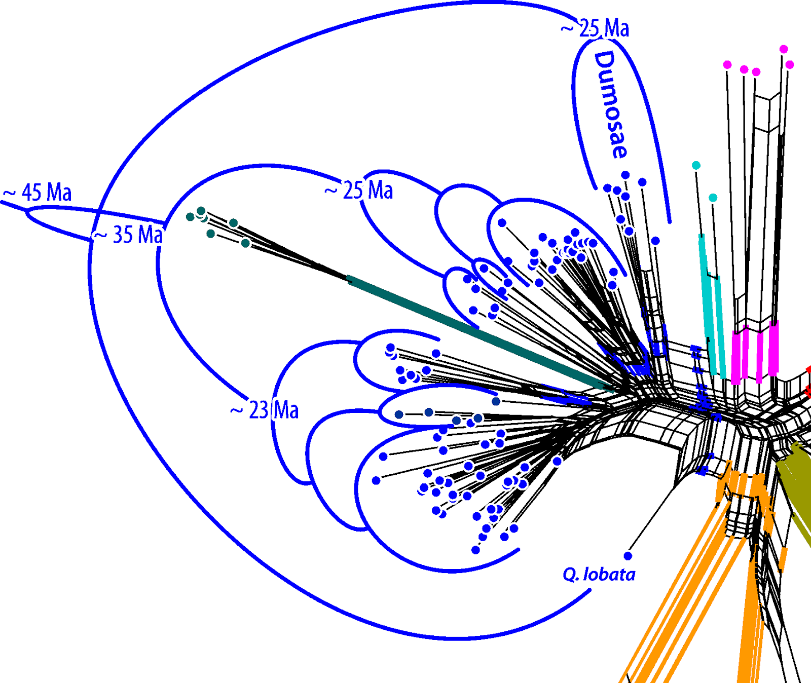
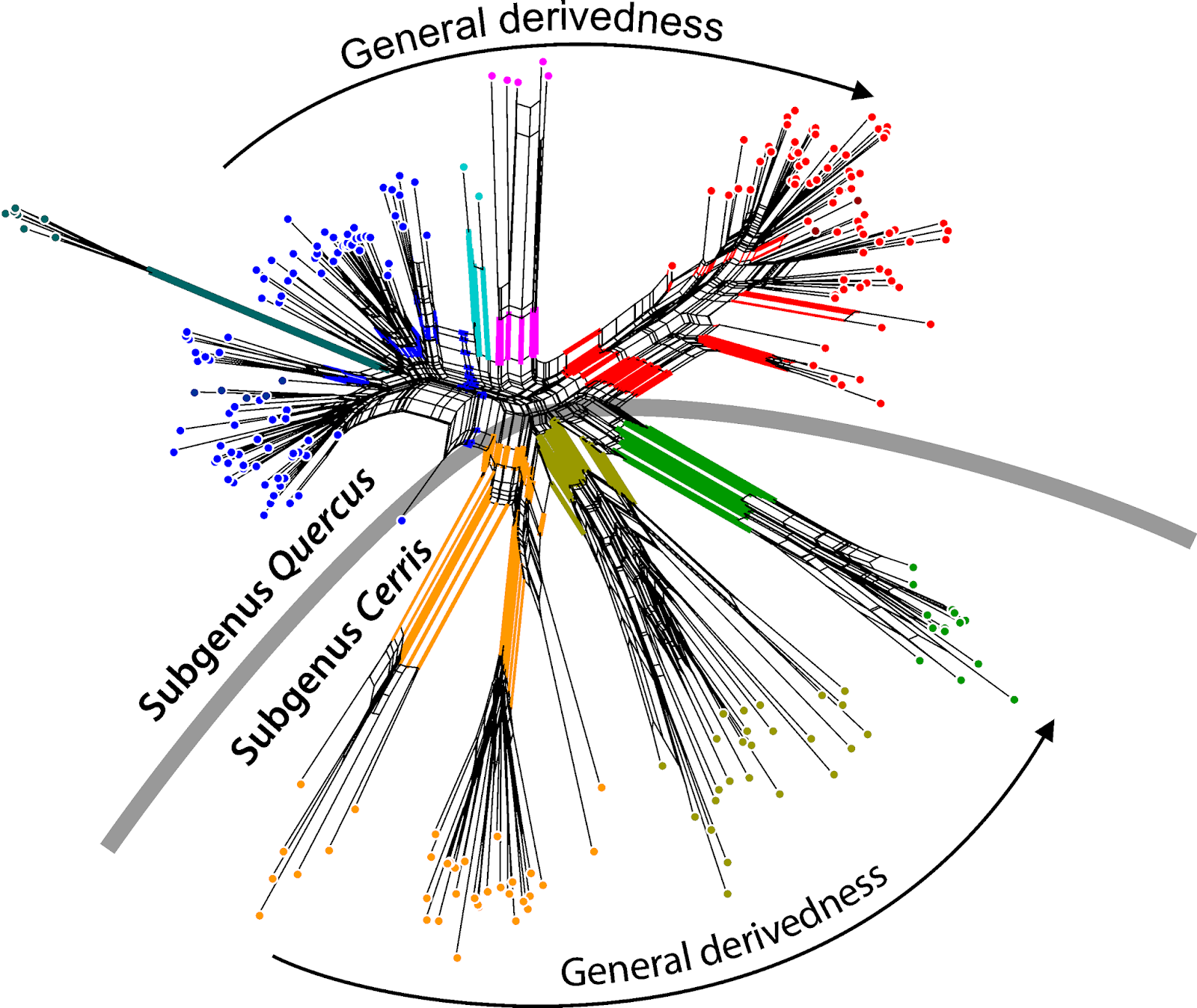
If the data follows two incongruent trees ("phylogenies"), as in this case for the oaks, the Neighbor-net has a good chance of capturing the incompatible splits of both genealogies. Here is the graph from the paper.

Wang et al.'s fig. 1b.

The central inflated portion of the graph reflects the incongruence between the combined data sets: we have overlapping nuclear-informed and plastid-informed neighborhoods.

The authors' brackets (shown in black) refer to neighborhoods triggered by the two nuclear markers in the data set: these are neighborhoods reflecting the common origin and speciation within the oak lineages. We can even see that this signal, which is incompatible with all deep splits in the combined tree, is unambiguous in part of the data (the nuclear partitions): section Ilex spans out as a wide fan, but there is a relatively prominent edge bundle defining the according neighborhood (the blue split).

The net shows additional, even more prominent edge bundles defining partly overlapping or distinct neighborhoods (the red splits). These neighborhoods are represented as clades in Yang et al.'s phylogenetic tree (fig.1a). They write (p. 11 of 20):
However, the conflict between the two datasets seems to be recovered by the neighbor-net method in this study, as the neighbor-net network based on combined plastid–nuclear data strongly shows the presence of two subgenera and four infrageneric species groups for the Chinese oak’s lineage (Figure 1b).
Interestingly, the authors nonetheless used the substantially incongruent combined data for downstream dating and trait mapping analysis (p. 7/20):
Bayesian evolutionary analyses provided a concordant infrageneric phylogeny for the Chinese oak’s lineage at the species level (Figure 2).
This uses a taxon-filtered, obviously constrained (fixed) topology, fitted to the current synopsis outlined in Denk et al. (2017). [Note: the supplement includes the extremely incongruent nuclear and plastid trees, each of which has further incongruence issues because they combine fast- and very slow-evolving sequence regions.]

Postscript

More posts on oaks, plastid data and networks can be found here in the Genealogical World and in my Res.I.P. blog.

Cited papers

Denk T, Grimm GW, Manos PS, Deng M, Hipp AL. (2017) An updated infrageneric classification of the oaks: review of previous taxonomic schemes and synthesis of evolutionary patterns. In: Gil-Pelegrín E, Peguero-Pina JJ, and Sancho-Knapik D, eds. Oaks Physiological Ecology. Cham: Springer, pp. 13–38. Open access Pre-Print [major change: Ponticae and Virentes accepted as additional sections in final version].

Hipp AL, Manos PS, Hahn M, Avishai M, + 20 more authors. (2020) Genomic landscape of the global oak phylogeny. New Phytologist 229: 1198–1212. Open access.

Simeone MC, Grimm GW, Papini A, Vessella F, Cardoni S, Tordoni E, Piredda R, Franc A, Denk T. (2016) Plastome data reveal multiple geographic origins of Quercus Group Ilex. PeerJ 4:e1897. Open access.

Yan M, Liu R, Li Y, Hipp AL, Deng M, Xiong Y. (2019) Ancient events and climate adaptive capacity shaped distinct chloroplast genetic structure in the oak lineages. BMC Evolutionary Biology 19:202. Open access.


** The publisher, MDPI, thrives in the gray zone between predatory and accredited publishing. Originally included in the recently reactivated Beall's List (new homepage), it has been tentatively dropped (see the linked Wikipedia article; but see also this post by Mats Widgren). Personally, I have encountered articles published in MDPI journals only where the review process must have been, at least, strongly compromised. But it's always quick: Yang et al.'s paper was submitted July 24th, accepted August 12th, and published a day later. Three weeks is about the length of time that the editors of my first oak paper needed to find a peer reviewer at all.

Large morphomatrices – trivial signal


In my last post about fossils, Farris and Felsenstein Zones, I gave an example of a trivial (signal-wise perfect) binary phylogenetic matrix, which will give us the true tree no matter which optimality criterion we use. In this post, we will look at a real world example, a huge bird therapods matrix.
S. Hartman, M. Mortimer, W. R. Wahl, D. R. Lomax, J. Lippincott, D. M. Lovelace
A new paravian dinosaur from the Late Jurassic of North America supports a late acquisition of avian flight. PeerJ 7: e7247.
What intrigued me about this particular paper (I have no idea about dinosaurs, but the documentation, pictures and data, and presentation seems impeccable) was the following sentence:
The analysis resulted in >99999 most parsimonious trees with a length of 12,123 steps. The recovered trees had a consistency index of 0.073, and a retention index of 0.589.
What can you possibly do with strict consensus trees (Losing information in phylogenetic consensus) based on an unknown number of MPTs that have a CI converging to 0 (but and RI of 0.6; The curious case[s] of tree-like matrices with no synapomorphies)? And isn't this a case for some networks-based exploratory data analysis?

The complete matrix has 501 taxa and 700 characters (the largest plant morphological matrices have hardly more than 100 characters) but also a gappyness of 72%. In this case, 255,969 of the 353,500 cells in the matrix are ambiguous or undefined (missing). The matrix is a (rich) Swiss cheese with very big holes. The high number of MPTs is hence not surprising, and neither is the low CI.

Why run elaborate tree-inferences on such a swiss cheese matrix? One answer is that (some) vertebrate palaeophylogeneticists are convinced that few taxa – many character matrices can lead to wrong clades (clades that are not monophyletic); and each added taxon, no matter how many characters can be scored, will lead to a better tree, by eliminating (parsimony) branching artifacts (see Q&A to the paper). At least 56 of the 501 taxa have 5% or fewer defined characters; still, with 700 characters, 5% equals up to 35 defined traits, which is more than we can recruit for most plant fossils. The median missing data proportion is 74% — more than half of the taxa are scored for less than 26% (< 182 out of 700) of the characters. Can such taxa really save the all-inclusive tree from branching artefacts, or is the high number of MPTs an indication for signal conflicts and data gaps issues?

For this post, we will just look at the tip of the iceberg. What is the signal from the 700 characters to start with?

The basic signal

Here's the heat map for the 19 taxa that have a gappyness of less than 15% (ie. at least 595 of 700 possible characters are defined). The taxon order is mostly the one from the original matrix, sorted by phylogenetic groups — for more orientation, I added next-inclusive superclass "Clades" from Wikipedia (so apologize any errors).


In my last post, I showed that evolutionary lineages (and monophyly) can be directly deduced from such a heat map following the simple logic: two taxa sharing a (direct) common origin are usually more similar to each other than to a third, fourth etc. taxon not part of the same lineage. Exceptions include fossils close to the last common ancestors lacking advanced traits.

The outgroup as used (in this taxon sample: Allosaurus to Tyrannosaurus) is most similar to each other but not monophyletic. One (Allosaurus) respresents the sister lineage of, the other an early split within the lineage that lead to the birds (Coelurosauria:Tyrannoraptora). The extinct (monophyletic) families (Tyrannosauridae, Ornithomimidae, Dromaesauridae) are, however, well visible, being defined by low intra-family and higher inter-family pairwise distances. The same is true for the direct relatives (Clade Ornithurae) of modern birds (class Aves).

Very typical for such datasets is the increasing distance between the (primitive?) outgroups and the most derived, modern-day taxa (living birds: Struthio – ostrich, Anas – duck, Meleagris – turkey). Closest relatives in the taxon set, phylogenetically and time-wise, are (much) more similar than distant ones. Allosaurus may be most similar to the tyrannosaurs, not because of common ancestry but because both are scored as being primitive with respect to the group of interest.

The only tree

This situation becomes very obvious from the only possible (single-optimal) tree that can be inferred from this matrix, when visualized as a phylogram (Stop using cladograms!)

The ML, MP and LS/NJ tree overlapped and scaled to equal root (first split within Tyrannoraptor) to tip (split between Anas and Meleagris) distance (phylogenetic distance, via the tree). Pink, the LS clade conflicting with ML and MP trees, and Wikipedia's tree(s).

No matter which optimisation criterion is used (here Least-Squares via Neighbor-joining, Maximum Parsimony, Maximum Likelihood), the result is the same. The only exception is that the NJ/LS tree places Archaeopteryx as sister to Dromaeosauridae; and the relative branch lengths of roots vs. tips also differ.

Because our matrix has favorable properties (few taxa, many defined characters), it's straightforward to establish branch support. This is a bit frowned upon in palaeontological circles, but having dealt with morphological evolution in cases where we have molecular data, I want to know how robust my clades are, and what may be the alternatives, before I conclude that they reflect monophyly. Bootstrapping coupled with consensus networks is a quick and simple way to test robustness and investigate ambiguous support (Connecting tree and network edges) .

The BS support consensus networks for NJ/LS and ML have only a single reticulation each.

Rooted support consensus networks based on the NJ/LS (10,000 pseudoreplicates, PAUP*) and ML bootstrap (100, number of necessary replicates determined by bootstop criterion implemented in RAxML) samples. Only splits are shown that ocurred in at least 15% of the BS pseudoreplicates.

The MP BS support consensus network is, however, has many more reticulations.

Rooted MP-BS support consensus network (10,000 BS pseudoreplicates, PAUP*). Green — edge bundles corresponding to clades in the all-optimal tree(s); orange — less supported conflicting alternatives; red – higher supported conflicting alternatives; pink – wrong clade in NJ/LS tree.

We can make two generally relevant observations here:
  1. The wrong Archaeopterix-Dromaeosauridae clade (pink edge/branch) masks a split BSNJ support: 68 for the wrong clade, 31 for the right one. While resampling under ML appears to be inert to this conflict, MP is not.
  2. While the NJ- and ML support networks are very tree-like, all clades in the inferred tree have high to unambiguous support, and are near-congruent, the MP network is much more boxy. In some cases the split in agreement with the all-optimal tree has a lower BS support than an alternative (here usually in conflict with the gold tree).
Similar observations can be made with other data sets: although NJ/LS and ML optimisation are fundamentally different (distance- vs. character-based, equal change vs. varying probability of change), they show more agreement with each other when it comes to supporting a topology (or topological alternatives) than MP (character-based like ML, but all changes are treated as equal like NJ/LS). MP is a very conservative approach, highly dependent on possibly a few discerning characters. If they are missing from the BS pseudoreplicate, the backbone tree collapses or changes, and BS values may decrease rapidly. This is so even for a very data-dense matrix like the one used here (few taxa, many characters, low gappyness).

On the positive side, we can expect that MP will produce fewer false positives. On the negative side, it is also more dependent on character coverage, and will produce much more false negatives. Any fossil lacking the crucial characters (or showing too few of them) may be still resolved (placed and supported) under NJ/LS and ML but not using MP. When inferring trees, these fossils will quickly increase the number of MPTs and decrease branch support for the part of the tree they interact with. Personally, given how hard it can be to place a fossil per se with the data at hand, I always preferred a method that can give some result, and point towards possible alternatives (even risking including erroneous), rather than no result at all.

The simplest of networks

Naturally, we can use the distance matrix directly to infer a Neighbor-net, and explore the basic differentiation signal beyond trees but also with regard to the all-optimal tree.

Neighbor-net based on the pairwise distance matrix. Coloration highlights edges found (or not) in the optimised trees.

The Neighbor-net recovers the clades from the all-optimal tree (green, purple the NJ/LS-unique branch), but shows additional edges (orange). The principal signal in the data has, for instance, problems with placing Archaeopteryx, because it is (signal-wise) intermediate between the Avebrevicaudata, the lineage including modern birds, and the Dromaeosauridae, their sister lineage (note that the vertebrate fossil record is considered to be free of ancestors and precursors; all fossils represent extinct sister lineages – evolutionary dead-ends). Skeleton IGM 100042 (an Oviraptoridae), placed as sister to both in the all-optimal tree, also lacks obvious affinities: this is a taxon where the tree inference makes a decision that is not based on a trivial signal encoded in the matrix.

The central boxy part of the Neighbor-net correlates with the 2/3-dimensional part of the parsimony BS consensus network: to resolve these relationships, we need a large set of characters (under MP). On the other hand, recognizing the Ornithurae, members of an extinct family, or a relative of IGM 100042, should be straightforward even with a limited amount of defined characters. Based on the Neighbor-net, which is inferred in a blink no matter how large the matrix, we can also make a decision, as to which taxa interfere and which ones facilitate tree-inferences. The more tree-like the Neighbor-net graph becomes, the easier it is for a tree inference to be made.

Placing fossils, quickly and easily

Using this backbone graph, it is easy to assess in which phylogenetic neighborhood a newly coded fossil falls, eg. the fossil newly described in Hartman et al. and scored for 267 unambiguously defined traits, Hesperornithoides.

Neighbor-net including Hesperornithoides.

Hesperornithoides is obviously a member of the Eumaniraptora (= Paraves), morphologically somewhat intermediate between the Avialae, the "flying dinosaurs", and Dromaeosauridae, but doesn't seem to be part of either of these sister lineages. The graph lacks a prominent neighborhood, the Archaeopteryx-Bambiraptor neighborhood may reflect local long-edge attraction (note the long terminal edges) or convergent evolution in both taxa and, possibly, also the Hesperornithoides lineage. Just based on this simple and quick-to-infer network, Hartman et al.'s title "A new paravian dinosaur from the Late Jurassic of North America supports a late acquisition of avian flight" appears to be correct (in future posts, we may come back to this morphological supermatrix to see what else networks could have quickly shown).

One should be willing to leave the phylogenetic beaten track – ie. relying on strict consensus parsimony trees as the sole basis for phylogenetic hypothesis. The Neighbor-net is a valuable tool for quick pre- and post-analysis because it can:
  • visualize how coherent the clades in our trees are, 
  • how easy it will be for the tree inference (especially MP) to find and support clades, 
  • help to differentiate ambiguous from important taxa, and finally, 
  • assess whether a new fossil really requires an in-depth re-analysis of the full matrix (and dealing with >99,999 MPTs) instead of using a more focussed taxon (and character) set.

Character cliques and networks – mapping haplotypes of manual alphabets


[This post is the second part of our miniseries on the origin and evolution of sign language manual alphabets]

One aspect of exploratory data analysis (EDA) is for us to try to understand how our data relate to our inference(s). This is especially important when the signal from our data is increasingly complex. Sign language manual alphabets are such a case.

In our first post about sign language manual alphabets, I introduced the principal networks that we used to classify sign languages. Here, I'll describe our character mapping procedure and why we did it as part of our EDA framework, in order to establish scenarios for the origin and evolution of sign languages.

Characters and mapping

We encoded each hand-shape used to signify a certain concept, such as the letters included in the standard Latin alphabet "a", "b", "c", .... "x", "y", "z", as a binary sequence – the presence or absence of a certain COGID (we will explain and discuss this in a later post). These binary sequences can be seen as an analogy of the genetic code, as a sort of 'linguistic haplotype', and their evolution can be mapped onto a network based on the entire dataset.

For instance, our matrix has three binaries (haplotypes) for the concept [g] in the oldest set of sign languages (pre-1840), two of which can be found in the earliest alphabets in our dataset: those of Yebra 1953 and Bonet 1620. Russian 1835, the oldest Cyrillic alphabet, uses a somewhat different hand-shape for its counterpart of the Latin "g", the Cyrillic "г".

For the concept [g], we thus have three taxon cliques, each defined by a distinct binary/haplotype: the 'Yebra haplotype', the 'Bonet haplotype', and the 'Cyrillic haplotype'.

By mapping these haplotypes on the network, as shown in the next figure, we can see that there is a small edge bundle reflecting the basic split between the Yebra and Bonet haplotypes.

Hand-shape drawings are taken from the original manuscripts.

We can also see that the Russian haplotype either evolved from the Yebra haplotype kept in the older Austrian-origin Group, ie. is an adaptation of the Yebra haplotype, or that it is a genuinely new invention — note the similarity of the Russian hanshape with the letter г.

We repeated this procedure for all 26 concepts of the standard Latin alphabet, to get an idea of how often the encoded linguistic haplotypes fit with the overall pattern visualized in the inferred Neighbor-nets (ie. the neighborhoods as defined by edge bundles). This is shown in the next figure.

The arrows indicate inferred evolutionary processes (replacement or invention).

Using this network mapping(which, in principle, uses the logic of parsimony/median networks), we can make direct inferences about the general mode of evolution.

For instance, even though Russian 1835 uses a different set of hand-shapes (ie. is defined by partly unique haplotypes), the hand-shapes for the concepts [p] and [z] are exclusively shared with the Austrian-origin Group. The biological equivalent would be: the 'Austrian haplotypes' are a uniquely shared derived feature reflecting a putative common origin of the Austrian and Russian lineages — ie a potential linguistic synapomorphy. We also can see that all haplotypes shared by Russian and all ([a][c][f][r][u][y]) or part ([b][e][i][k][n][o][x]) of the French-origin Group, an alternative source that may have inspired this early Cyrillic alphabet, lack this quality.

We can also make inferences about:
  1. which hand-shape is the original one (O);
  2. lineage-specific / diagnostic hand-shapes, eg. At. = Austrian, Da. = Danish (using two letter abbreviations);
  3. which hand-shapes are shared but apparently derived, eg. At.-Fr. are hand-shapes / haplotypes shared by members of the Austrian- and French-origin groups not found in the Yebra or Bonet alphabets — C stands for cosmopolitan, non-original handshapes common in various lineages, including British-origin Group, and D represents derived but rare hand-shapes without any clear lineage-affiliation; and
  4. alphabet-unique (ie. represent a linguistic autapomorphy.
In addition, we can explore certain details, including patterns (character-based taxon cliques) that are at odds with the overall reconstruction. The latter are to be expected, because the graph is planar (2-dimensional) but the processes that shaped sign alphabets are likely to be multi-dimensional. For instance, our networks failed to resolve the affinity of the contemporary Norwegian Sign Language, the reason for which can be seen in the following character map.


Note the position of Norwegian 1955, which is still part of the Austrian-origin Group (like older manual alphabets used in the late 19th century in Norway). However, it is already influenced by international standardization — eg. concepts [k], [p], and [z] use(d) French hand-shapes. Hence, Norwegian 1955 shares quite a high number of lineage-diagnostic hand-shapes with Danish 1967 and the Icelandic Sign Language. These, and others, were further replaced in its contemporary counterpart (Norwegian SL) by hand-shapes borrowed from various lineages — eg. [c],[f] from the nearly extinct Austrian-origin Group, [p] from the Russian Group, [k] same as in the Spanish Group) — as well as unique hand-shapes, including hand-shapes evolved from earlier forms or those that have been genuinely invented.

Why we map character evolution along networks

In many cases, we only have one set of data, in order to draw our conclusions based on the graph(s) we infer. We cannot test to which degree our data (the way we scored the differentiation patterns) and inferences are systematically biased. Thus, we want to explore which aspects of our inference are supported by character splits, and establish taxon cliques and evolutionary pathways for the characters (scored traits). Lacking an independent source of data, the latter would involve circular reasoning — ie. mapping the traits along a tree derived from those same traits.

By inferring a tree, we crystallize one pattern dimension out of the data, although more often than not this will be a comprise from multidimensional signals. A network, such as a Neighbor-net, has two dimensions, and hence our mapping can consider two alternatives at the same time — this enables us to make a choice, if we have to. Another practical advantage of a Neighbor-net is that it is quick to infer, so that we can easily reduce the data set and use a more focused graph for the map.

In cases where 2-dimensional graphs don't suffice, there are still Consensus networks, which would allow mapping character evolution based on a sample of many alternative trees.

We could even eliminate the circular reasoning while maintaining a relatively stable inference framework. Deleting a character or several characters (or recoding them: see eg. Should we try to infer trees on tree-unlikely matrices?) can easily lead to a new tree topology, although it has less effect on the structure of a Neighbor-net. When we would need to worry about circular reasoning for mapping a certain concept, or two concepts that may have interacted, we just base our Neighbour-net on a distance matrix calculated from a reduced character matrix, and then map only those concepts not considered for the inference.

Other posts in this miniseries

Next-generation neighbor-nets


Neighbor-nets are a most versatile tool for exploratory data analysis (EDA). Next-generation sequencing (NGS) allows us to tap into an unprecedented wealth of information that can be used for phylogenetics. Hence, it is natural step to combine the two.

I have been waiting for it (actively-passively) and the time has now come. Getting NGS data has become cheaper and easier, but one still needs considerable resources and fresh material. Hence, NGS papers usually not only use a lot of data, but also are many-authored. You can now find neighbor-nets based on phylogenomic pairwise distances computed from NGS data — for example, in these two recently published open access pre-prints:
  • Pérez Escobar​ OA, Bogarín D, Schley R, Bateman R, Gerlach G, Harpke D, Brassac J, Fernández-Mazuecos M, Dodsworth S, Hagsater E, Gottschling M, Blattner F. 2018. Resolving relationships in an exceedingly young orchid lineage using Genotyping-by-sequencing data. PeerJ Preprint 6:e27296v1
  • Hipp AL, Manos PS, Hahn M, Avishai M, Bodénès C, Cavender-Bares J, Crowl A, Deng M, Denk T, Fitz-Gibbon S, Gailing O, González Elizondo MS, González Rodríguez A, Grimm GW, Jiang X-L, Kremer A, Lesur I, McVay JD, Plomion C, Rodríguez-Correa H, Schulze E-D, Simeone MC, Sork VL, Valencia Avalos S. 2019. Genomic landscape of the global oak phylogeny. bioRxiv DOI:10.1101/587253.

Example 1: A young species aggregate of orchids

Pérez Escobar et al.'s neighbor-nets are based on uncorrected p-distances inferred from a matrix including 13,000 GBS ("genotyping-by-sequencing") loci (see the short introduction for the method on Wikipedia, or the comprehensive PDF from a talk at/by researchers of Cornell) covering 29 accessions of six orchid species and subspecies.

They also inferred maximum likelihood trees, and did a coalescent analysis to consider eventual tree-incompatible signal, gene-tree incongruence due to potential reticulation and incomplete lineage sorting. They applied the neighbor-net to their data because "split graphs are considered more suitable than phylograms or ultrametric trees to represent evolutionary histories that are still subject to reticulation (Rutherford et al., 2018)" – which is true, although neighbor-nets do not explicitly show a reticulate history.

Here's a fused image of the ML trees (their fig. 1) and the corresponding neighbor-nets (their fig. 2):

Not so "phenetic": NGS data neighbor-nets (NNet) show essentially the same than ML trees — the distance matrices reflect putative common origin(s) as much as the ML phylograms. The numbers at branches and edges show bootstrap support under ML and the NNet optimization.

Groups resolved as clades, Group I and III, or grades or clades, Group II (compare A vs. B and C), in the ML trees form simple (relating to one edge-bundle) or more complex (defined by two partly compatible edge-bundles, Group I in A) neighborhoods in the neighbor-net splits graphs. The evolutionary unfolding, we are looking at closely related biological units, was likely not following a simple dichotomizing tree, hence, the ambiguous branch-support (left) and competing edge-support (right) for some of the groups. Furthermore, each part of a genome will be more descriminative for some aspect of the coalescent and less for another, another source of topological ambiguity (ambiguous BS support) and incompatible signal (as seen in and handled by the neighbor-nets). The reconstructions under A, B and C differ in the breadth and gappyness of the included data (all NGS analyses involve data filtering steps): A includes only loci covered for all taxa, B includes all with less than 50% missing data, and C all loci with at least 15% coverage.

PS I contacted the first author, the paper is still under review (four peers), a revision is (about to be) submitted, and, with a bit of luck, we'll see it in print soon.


Example 2: The oaks of the world

The Hipp et al. (note that I am an author) neighbor-net is based on model-based distances. The reason I opted (here) for model-based distance instead of uncorrected p-distances is the depth of our phylogeny: our data cover splits that go back till the Eocene, but many of the species found today are relatively young. The dated tree analyses show substantial shifts in diversification rates. In the diverse lineages today and possibly in the past (see the lines in the following graph), in those with few species (*,#) we may be looking at the left-overs of ancient radiations.

A lineage(s)-through-time plot for the oaks (Hipp et al. 2019, fig. 2). Generic diversification probably started in the Eocene around 50 Ma, and between 10–5 Ma parts (usually a single sublineage) of these long-isolated intrageneric lineages (sections) underwent increased speciation.

The data basis is otherwise similar, SNPs (single-nucleotide polymorphisms) generated using a different NGS method, in our case RAD-tagging (RAD-seq) of c. 450 oak individuals covering the entire range of this common tree genus — the most diverse extra-tropical genus of the Northern Hemisphere. There are differences between GBS and RAD-seq SNP data sets — a rule of thumb is that the latter can provide more signal and SNPs, but the single-loci trees are usually less decisive, which can be a problem for coalescent methods and tests for reticulation and incomplete lineage sorting that require a lot of single-loci (or single-gene) trees (see the paper for a short introduction and discussion, and further references).

We also inferred a ML tree, and my leading co-authors did the other necessary and fancy analyses. Here, I will focus on the essential information needed to interpret the neighbor-net that we show (and why we included it at all).

Our fig. 6. Coloring of main lineages (oak sections) same as in the LTT plot. Bluish, the three sections traditionally included in the white oaks (s.l.); red, red oaks; purple, the golden-cup or 'intermediate' (between white and red) oaks — these three groups (five sections) form subgenus Quercus, which except for the "Roburoids" and one species of sect. Ponticae is restricted to the Americas. Yellow to green, the sections and main clades (in our and earlier ML trees) of the exclusively Eurasian subgenus Cerris.

Like Pérez Escobar et al., we noted a very good fit between the distance-matrix based neighbor-net and the optimised ML tree. Clades with high branch support and intra-clade coherence form distinct clusters, here distinct neighborhoods associated with certain edge bundles (thick colored lines). This tells us that the distance-matrix is representative, it captures the prime-phylogenetic signal that also informs the tree.

The first thing that we can infer from the network is that we have little missing data issues in our data. Distance-based methods are prone to missing data artifacts and RAD-seq data are (inevitably) rather gappy. It is important to keep in mind that neighbor-nets cannot replace tree analysis in the case of NGS data, they are "just" a tool to explore the overall signal in the matrix. If the network has neighborhoods contrasting what can be seen in the tree, this can be an indication that one's data is not sufficiently tree-like at all. But it also can just mean that the data is not sufficient to get a representative distance matrix.

Did you notice the little isolated blue dot (Q. lobata)? This is such a case — it has nothing to do with reticulation between the blue and the yellow edges, it's just that the available data don't produce an equally discriminative distance pattern: according to its pairwise distances, this sample is generally much closer to all other oak individuals included in the matrix in contrast to the other members of its Dumosae clade, which are generally more similar to each other, and to the remainder of the white oaks (s.str., dark blue, and s.l., all bluish).

Close-up on the white oak s.str. neighbor-hood (sect. Quercus) and plot of the preferred dated tree.

In the tree it is hence placed as sister to all other members, and, being closer to the all-ancestor, it triggers a deep Dumusae crown age, c. 10 myr older than the subsequent radiation(s) and as old as the divergence of the rest of the white oaks s.str.

The second observation, which can assist in the interpretation of the ML tree (especially the dated one), is the principal structure (ordering) within each subgenus and section. The neighbor-net is a planar (i.e. 2-dimensional graph), so the taxa will be put in a circular order. The algorithm essentially identifies the closest relative (which is a candidate for a direct sister, like a tree does) and the second-closest relative. Towards the leaves of the Tree of Life, this is usually a cousin, or, in the case of reticulation, the intermixing lineage. Towards the roots, it can reflect the general level of derivation, the distance the (hypothetical all-)ancestor.

Knowing the primary split (between the two subgenera), we can interprete the graph towards the general level of (phylogenetic) derivedness.

The overall least derived groups are placed to the left in each subgenus, and the most derived to the right. The reason is long-branch attraction (LBA) stepping in: the red and green group are the most isolated/unique within their subgenera, and hence they attract each other. This is important to keep in mind when looking at the tree and judge whether (local) LBA may be an issue (parsimony and distance-methods will always get the wrong tree in the Felsenstein Zone, but probabilistics have a 50% chance to escape). In our oak data, we are on the safe side. The red group (sect. Lobatae, the red oaks) are indeed resolved as the first-branching lineage within subgenus Quercus, but within subgenus Cerris it is the yellow group, sect. Cyclobalanopsis. If this would be LBA, Cyclobalanopsis would need to be on the right side, next to the red oaks.

The third obvious pattern is the distinct form of each subgraph: we have neighborhoods with long, slim root trunks and others that look like broad fans.

Long-narrow trunks, i.e. distances show high intra-group coherence and high inter-group distinctness can be expected for long isolated lineages with small (founder) population sizes, eg. lineages that underwent in the past severe or repeated bottleneck situations. Unique genetic signatures will be quickly accumulated (increasing the overall distance to sister lineages), and the extinction ensures only one (or very similar) signature survives (low intragroup diversity until the final radiation).

Fans represent gradual, undisturbed accumulation of diversity over a long period of time, eg. frequent radiation and formation of new species during range and niche expansion – in the absence of stable barriers we get a very broad, rather unstructured fan like the one of the white oaks (s.str.; blue); along a relative narrow (today and likely in the past) geographic east-west corridor (here: the  'Himalayan corridor') a more structured, elongated one as in the case of section Ilex (olive).

Close-up on the sect. Ilex neighborhood, again with the tree plotted. In the tree, we see just sister clades, in the network we see the strong correlation between geography and genetic diversity patterns, indicating a gradual expansion of the lineage towards the west till finally reaching the Mediterranean. Only sophisticated explicit ancestral area analysis can possibly come to a similar result (often without certainty) which is obvious from comparing the tree with the network.

This can go along with higher population sizes and/or more permeable species barriers, both of which will lead to lower intragroup diversity and less tree-compatible signals. Knowing that both section Quercus (white oaks s.str., blue) and Ilex (olive) evolved and started to radiate about the same time, it's obvious from the structure of both fans that the (mostly and originally temperate) white oaks produced always more, but likely less stable species than the mid-latitude (subtropical to temperate) Ilex oaks today spanning an arc from the Mediterranean via the southern flanks of the Himalayas into the mountains of China and the subtropics of Japan.

Networks can be used to understand, interpret and confirm aspects of the (dated) NGS tree.

The much older stem and young crown ages seen in dated trees may be indicative for bottlenecks, too. But since we typically use relaxed clock models, which allow for rate changes and rely on very few fix points (eg. fossil age constraints), we may get (too?) old stem and (much too) young crown ages, especially for poorly sampled groups or unrepresentative data. By looking at the neighbor-net, we can directly see that the relative old crown ages for the lineages with (today) few species fit with their within-lineage and general distinctness.

The deepest splits: the tree mapped on the neighbor-net.

By mapping the tree onto the network, and thus directly comparing the tree to the network, we can see that different evolutionary processes may be considered to explain what we see in the data. It also shows us how much of our tree is (data-wise) trivial and where it could be worth to take a deeper look, eg. apply coalescent networks, generate more data, or recruit additional data. Last, but not least, it's quick to infer and makes pretty figures.

So, try it out with your NGS data, too.

PS. Model-based distances can be inferred with the same program many of us use to infer the ML tree: RAxML. We can hence use the same model assumptions for the neighbor-net that we optimized for the inferring tree and establishing branch support.