More heretic bits: networks for (more) recent matrices published in Cladistics


This is Part 2 of a 2-part blog series. Part 1 covered some history, while this post has three (more) recently published matrices, and the take-home message.

Jumping forward in time, welcome to the 21st century

In Part 1, I showed several networks generated based on some early phylogenetic matrices published in the first volumes of the journal Cladistics. In this post, we will look at the most recent data matrices and trees uploaded to TreeBASE, covering the past seven years.

Nearly a generation later, and facing the "molecular revolution", some researchers (fortunately) still compile morphological matrices. This is an often overlooked but important work: genes and genomes can be sequenced by machines, and the only thing we need to do is to feed these machine-generated data into other powerful machines (and programs) to get a phylogenetic tree, or network. But no software and computer cluster can (so far) study anatomy, and generate a morphological matrix. The latter is paramount when we want to put fossils, usually devoid of DNA, in a (molecular) phylogenetic context. We need to do this when we aim to reconstruct histories in space and time.

Nevertheless, we can't ignore the fact that these important data are (still) far from tree-like. What holds for the matrices of the 80's (see the end of Part 1), still applies now.

So, let's have a look at the three most recent data sets (one morphological, two molecular) published in Cladistics that have their data matrix in TreeBASE.

The morphological dataset

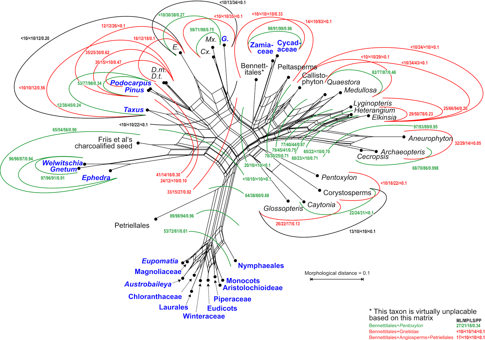
Beutel et al. (2011; submission S11976) provided a "robust phylogeny of ... Holometabola", and note in their abstract: "Our results show little congruence with studies based on rRNA, but confirm most clades retrieved in a recent study based on nuclear genes."

Without having read the study, I can guess which clades (likely used here as a synonym for monophyletic group; but see David's post on Hennig and Cladistics) were confirmed. The data matrix contains: 356 multistate, with up to six states, characters scored and annotated for 34 taxa, including polymorphisms and some gaps ("–") viz missing data ("?"). Just by looking at the Neighbor-net inferred from this matrix. (Standard tree- or network-inference doesn't differ between gaps and missing data, but some people find it important to distinguish between "not applicable" and "not known" in a matrix.)

Neighbor-net inferred from simple pairwise distances computed based on Beutel et al.'s matrix. Brackets show my ad hoc assessment of candidates for monophyla (here: likely represented by clades in no matter how optimized trees).

How did I postulate the monophyla? By deduction: if two or more OTUs are much more similar to each other than to anything else in the matrix, they likely are part of the same evolutionary lineage, ie. have a common origin (= monophyletic in a pre-Hennigian sense). This, when the matrix well covers the group and morphospace, has a good chance to be inclusive (= monophyletic fide Hennig; for the covered OTUs). This is especially so when there is a good deal of homoplasy — the provided tree has a CI of 0.44 and RC of 0.33: convergences should be more randomly distributed than lineage-specific/-conserved traits. The latter don't need to be (or were, at some point in time) synapomorphies, shared derived unique traits, but could be diagnostic suites of characters that evolved in parallel within a lineage and passed on to all (or most) of the descendants.

The first molecular dataset

Let's look at the signal in the two molecular matrices.

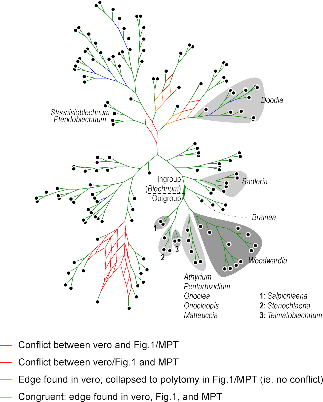
In 2016, Gaspar and Almeida (submission S19167) tested generic circumscriptions in a group of ferns by "assembl[ing] the broadest dataset thus far, from three plastid regions (rbcL, rps4-trnS, trnL-trnF) ... includ[ing] 158 taxa and 178 newly generated sequences". They found: "three subfamilies each corresponding to a highly supported clade across all analyses (maximum parsimony, Bayesian inference, and maximum likelihood)."

The total matrix has 3250 characters, of which 1641 are constant and 1189 are parsimony-informative. This is a quite a lot for such a matrix, and, by itself, rules out parsimony for tree-inference. If half of the nucleotide sites are variable, then the rate of character change was high, and parsimony is statistically only robust, when the rate of change was low. High mutation rates or high level of divergence may also pose problems for distance methods and other optimality criteria, all closely related to parsimony.

The file includes three trees, labelled "vero" (which, in Italian, means "true"), "Fig._1" and "MPT". "Vero" and "Fig._1" come with branch lengths; judging from the values (<< 1), they are probabilistic trees (of some sort); the "MPT" is (as usual) provided as a cladogram without branch-lengths. It may be that the authors had to add the parsimony tree just to fulfill editorial policies, while being convinced "vero" is the much better tree. "Vero" is a fully resolved tree (the ML tree?), while "Fig._1" (Bayesian?) and "MPT" include polytomies.

Using PAUP*'s "describe" function, we learn that the "MPT" is 5101 steps long and has a CI of 0.41 and RC of 0.33. Nucleotide sequence data can be notoriously homoplasious, as we repeat the same four states into infinity and have to deal with an unknown but usually significant amount of back mutations. This adds to the other problems for parsimony:
  • transitions are more likely to happen than transversions; and
  • in coding gene regions, such as the rbcL, some sites (3rd codon positions) mutate much faster than others.
Still, parsimony trees are not necessarily wrong. Neither are NJ trees; and there are also datasets where probabilistic methods struggle, eg. when the likelihood surface of the treespace is flat.

So, the first question is: how different are the three trees provided? Rather than having to show three graphs, we can show the (strict) Consensus network of those trees.

A strict consensus network summarizing the topologies of the three trees provided in the TreeBASE submission of

The main difference is between "vero" and the other two — "Fig. 1" and the "MPT" are very similar (and both include polytomies). There are three main scenarios for a Consensus network like this with respect to the high portion of variable sites:
  1. "Fig. 1" is a Jukes-Cantor model-based tree,
  2. "Fig. 1" is an uncorrected p-distance based tree, or
  3. most of the variation is between ingroup (the subtree including all Blechnum) and outgroup (the other subtree).
"Vero" is still quite congruent, so the model used here can't be too much different, either.

What should ring one's alarm bells are, however, the many grade-like / staircase subtrees, which are unusual for a molecular data set. Staircases imply that each subsequent dichotomous speciation event resulted in a single species and a further diversifying lineage: multiple, consistently occurring budding events.

The same graph, with arrows showing grade evolution. Often found in morpho-data-based trees with ancestral, more ancient, and derived (from them), modern forms, but should ring an alarm bell when common in a molecular tree. Major clades (found in all three trees) are labelled for comparison with the next graph.

Let's compare this to the Neighbor-net (usually, I would use model-based distances in such a case, but here we can do with uncorrected p-distances).

A Neighbor-net inferred from uncorrected p-distances based on Gaspar & Almeida's matrix; the major clades are labelled as in the preceding graph. Note the isolated, long-branch blue dots with asterisks, indicating the position of the first diverged species in the large clades G and I. Genuine signal or missing data artefact?

The Neighbor-net shows only a limited number of tree-like portions, but does correspond with the main clades above. Only A and B are dissolved, which are the two first diverging clades in the original trees (preceding graph). Some OTUs are placed close to the centre of the graph, or even along a tree-like portion (purple dots), a behaviour known from actual ancestors: some OTUs apparently have sequences that may be literally ancestral to others. This explains the grade structure seen in the original trees. Others (violet dots) create boxes, which may reflect a genuine ambiguous signal, or just be missing data leading to ambiguous pairwise distances. The latter (missing data artefact) is behind the misplacement of the four OTUs (red dots): missing data can inflate pairwise distances severely. And, like parsimony, distance-based methods are more vulnerable to long-branch(edge)-attraction than probabilistic methods.

Model-based distances may help clean up this a bit, but the networks needed for these kind of data are Support consensus networks (see e.g. Schliep et al., MEE, 2017). The split appearance of the Neighbor-net hints at internal signal conflict and, with respect to the high number of variable sites (note the sometimes extremely long terminal edges), saturation issues. Two major questions would be:
  1. How do the different markers (coding gene vs. inter-genic spacers with different levels of diversity; rps4-trnS is typically more divergent than the trnL-trnF spacer) resolve relationships, which clades / topological alternatives receive unanimous support?
  2. Does it make a difference to run a fully partitioned (ML) analysis vs. an unpartitioned one vs. one excluding the 3rd codon position in the gene?
For intra-clade evolutionary pathways, it would be worthwhile to give median networks and suchlike a try, as parsimony methods that can discern ancestor-descendant relationships.

The second molecular dataset

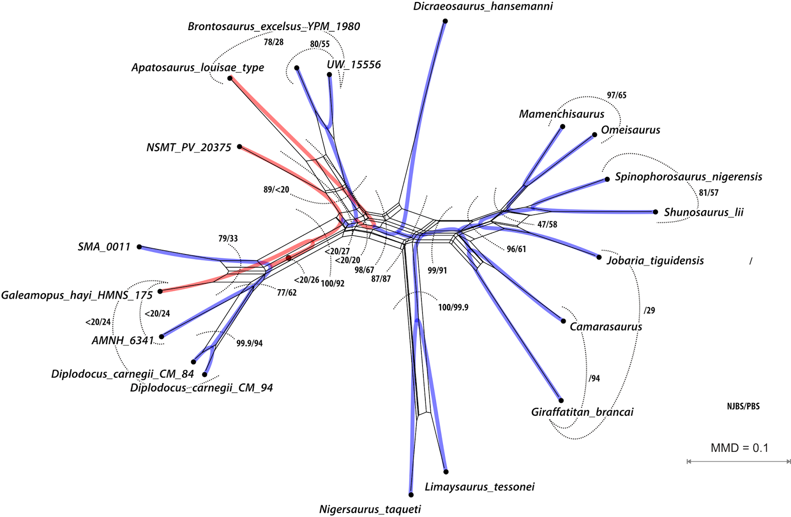
The most recent data are from Kuo et al. (2017; submission S20277), who inferred a "robust ... phylogeny" (see Part 1, Jamieson et al. 1987, and Beutel et al., above) for a group of ferns, focusing on the taxonomy of a single genus, Deparia, that now includes five traditionally recognized genera. In the abstract it says: "... seven major clades were identified, and most of them were characterized by inferring synapomorphies using 14 morphological characters".

The matrix includes the molecular characters used to infer the major clades plus two trees, labelled "bestREP1" and "rep9BEST", both with branch lengths. Branch length values indicate that "bestREP1" could be parsimony-optimized (with averaged or weighted branch lengths), while "rep9BEST" is either a ML or Bayesian tree (technically, it could be a distance-based tree, too, but I don't think such "phenetics" are condoned by Cladistics).

Re-calculated, the first tree ("bestREP1") is shorter (3024 steps) than the one of Gaspar & Almeida, reflecting the much lower number of parsimony-informative sites (979). Many of the sites differ only between the focal genus and the outgroups, which is well visible in the Neighbor-net. [For those of you unfamiliar with Neighbor-nets, a parsimony analysis of these data takes hours, or days depending on the software and computer, while the distance matrix and the resultant Neighbor-net is inferred in a blink.]

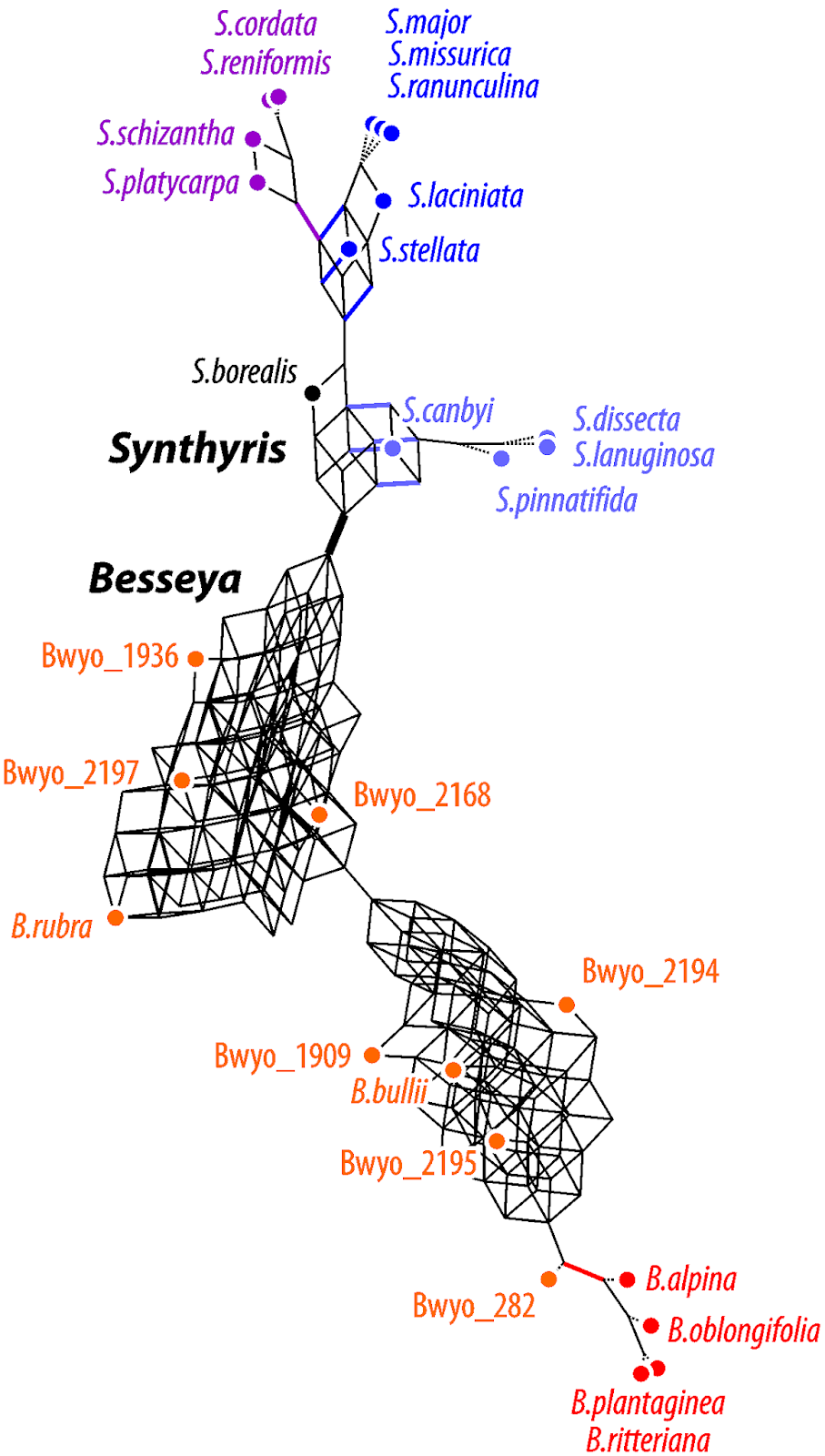
The Neighbor-net based on Kuo et al.'s data. Why do we need to include long-branching, distant outgroups when we just want to bring order in a genus? Because to test monophyly, we need a rooted tree (ambiguous or not, or even biased by branching artefacts).

Let's remove the distant, long-branching outgroups, which (as we can see in the Neighbor-net) at best provide ambiguous signal for rooting the ingroup — at worst, they trigger ingroup-outgroup branching artefacts. What could a Neighbour-net have contributed regarding taxonomy and the seven major monophyletic intrageneric groups ("clades")? Pretty much everything needed for the paper, I guess (judging from the abstract).

Same data as above, but outgroups removed. The structure of this Neighbour-net allows to identify seven likely candidates for monophyla ("1"–"7"), with "1" and "2" being obvious sister lineages. Colours refer to the clusters ("A"–"E") annotated above.

On a side note: by removing the long-branching, distant outgroups, taxon "T" is resolved as a probable member of the putative monophyletic group "5" (= "E" in the full graph with outgroups, and surely a high-supported subtree in any ingroup-only reconstruction, method-independent). Placing the root between "T" and the rest of the genus implies that "5" is a paraphyletic group comprising species that haven't evolved and diversified at all (ie. are genetically primitive), in stark contrast to the other main intra-generic lineages. This is not impossible, but quite unlikely. More likely is the second scenario (primary split between "1"–"3" and "4"–"7"). Having "4" as sister to the rest could be an alternative, too.

This is where Hennig's logic could be of help: find and tabulate putative synapomorphies to argue for a set and root that makes the most sense regarding morphological evolution and molecular differentiation.

The take-home message(s)

We have argued before that it is in the ultimate interest of science and scientists to give access to phylogenetic data. No matter where one stands regarding phylogenetic philosophy, we should publish our data, so that people can do analyses of their own. Discussion should be based on results, not philosophies.

When you deal with morphological data, you should never be content with inferring a single tree (parsimony or other). You have to use networks.

The Neighbor-net was born as late as 2002 (Bryant & Moulton, 2002, in: Guigó R, and Gusfield D, eds, Algorithms in Bioinformatics, Second International Workshop, WABI, p. 375–391; paywalled) and made known to biologists in 2004 (same authors, same title, in Mol. Biol. Evol. 21:255–265), so that authors before this time did not have access to its benefits. Similarly, Consensus networks arrived around about the same time (Holland & Moulton 2003, in: Benson G, and Page R, eds, Algorithms in Bioinformatics: Third International Workshop, WABI, p. 165–176). However, the Genealogical World of Phylogenetic Networks has been here for six years now (first post February 2012). So there is now no excuse for publishing a cladogram without having explored the tree-likeness of your matrix' signal!

Neighbor-nets like the ones I showed in this 2-piece post (or can be found in many of our other posts) are a quick and essential tool to explore the basic signal in your matrix:
  • How tree-like is it?
  • Where are the potential conflicts, obscurities?
  • What are the principal evolutionary alternatives (competing topologies)?
  • What is well supported (especially regarding taxonomy and the question of monophyly)?
Even if you don't use it in your paper, the network will tell you what you are dealing with when you start inferring trees.

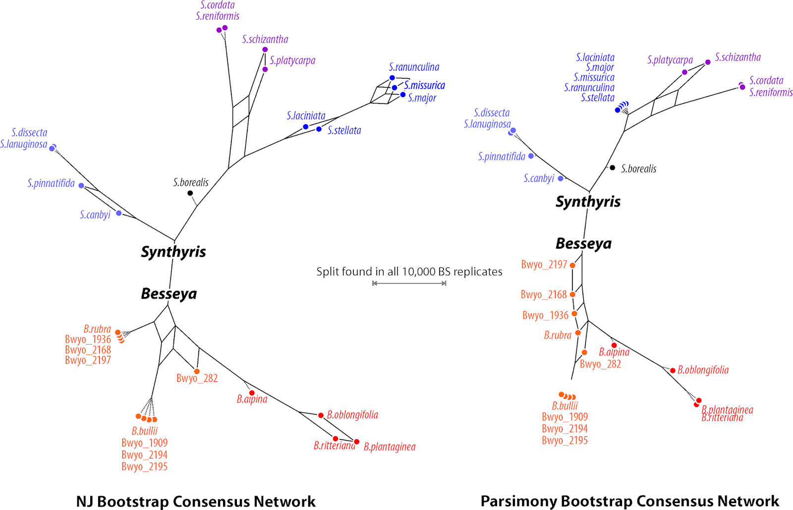
The second essential tool is the much under-used Support consensus network, not shown in this post but in plenty of our other posts (and many papers I co-authored; for a comprehensive collection of network-related literature see Who's who in phylogenetic networks by Philippe Gambette). Support consensus networks estimate and visualize the robustness of the signal for competing topological (tree) alternatives.

Consensus networks should also be obligatory for those molecular data,where even probabilistic methods fail to find a single fully resolved, highly supported tree.

If the editors of Cladistics are really dedicated to parsimony, they should not still insist only on a parsimony tree (often provided as cladogram), but also parsimony-based networks as well:
  • strict Consensus networks to summarize the MPT samples instead of the standard strict Consensus cladograms;
  • bootstrap Support consensus networks showing the signal strength and support for alternative trees/competing clades (TNT has many bootstrapping options to play around with); and
  • Median networks and such-like for datasets with few mutations, and low levels of expected homoplasy.
This is what the 2016 #parsimonygate uproar (see Part 1) should have been about (12 years after Neighbor-nets, and 11 years after Consensus networks). Not the prioritizing of parsimony, but the naivety or ignorance towards pitfalls of (parsimony or other) trees inferred from data not providing tree-like signal or riddled by internal conflict.
This is a problem not limited to Cladistics, but found, to my modest experience in professional science (c. 20 years), in many other journals as well (e.g. Bot. J. Linn. Soc., Taxon, Mol. Phyl. Evol., J. Biogeogr., Syst. Biol., Nature, Science).

Hence, here are my suggestions for future conference buttons, instead of those shown in Part 1.

No Cladograms!Use Neighbour-nets!Support Consensus Networks as obligatory!

Further reading for those who mistrust trees or become network-curious in general

A bit of heresy: networks for matrices used in Cladistics studies


[This is Part 1 of a two-part topic – this one is Historical matrices from the 1980s]

When I first came into contact with phylogenetics (usually based on morphological data sets, back then) and after reading Hennig's book (the original German version, published in 1950), I dreamed about publishing in Cladistics, the journal of the Willi Hennig Society (WHS). I never did. In this post, I show why.

Later on, in 2016, Cladistics achieved renewed fame due to an editorial that triggered a twitter uproar under the hashtag #parsimonygate. A lot of people were shocked to read in the editorial that the journal (still) prefers and requires parsimony-based inferences (in fact, parsimony-based trees). Some people, like Joe Felsenstein, were not at all surprised. I wasn't either, because Cladistics is the journal of the Willi Hennig Society (WHS), which has always been dedicated to parsimony: "Ockham told Popper told Hennig to use parsimony" (see the historical summary by Felsenstein in Systematic Biology, 2001; free access).

Historical buttons that you (allegedly) could get at meetings of the WHS. Left: Joe Felsenstein; right: L for Likelihood. Just a gag, of course! Nothing serious behind it.

In the good old days, when the "Phylogenetic Wars" were still on (in the 1980s, petering out in the 90s), they would invite a probability-ist to their conference to tear him down. My first phylogenetic paper (2002) got a negative review (ie. rejection, invitation to resubmit) by a WHS member solely because it did not include a parsimony tree, which he described as "standard these days". More recently, they ensured free access to TNT, the current main software for doing parsimony analysis and an essential tool for many palaeontologists.

I stopped using parsimony trees very early in my career, but I'm still a great fan of the family of methods based on median networks, which operate under the same parsimony criterion (Clades, Cladograms, ...; Using Median networks ...). Fate exposed me early to the Neighbor-nets, which can be used as a quick check of how tree-like the signal is in data matrices, to start with.

The thing that bugged me most concerning many journals, including Cladistics, is not a focus on parsimony, but the lack of data documentation and easy data access. To me, it seems natural to use a service like TreeBASE, when my main dedication is to tree-inference. TreeBASE allows you to provide your data and inferred trees to the general public in the common NEXUS format, so that other people can make use of it.

Luckily, some authors of Cladistics upload their data (about one study per 1–3 years). So, here are some data-display networks showing the strengths and weaknesses of the parsimony trees in the original publications, which have been randomly selected from among the oldest ones and the newest ones (I found) in TreeBASE. I won't discuss the actual results, as Cladistics is pay-walled, so just enjoy the graphs.

The oldest one (in my list), Dahlgren & Bremer 1985, TreeBASE submission number S231

The submission (a binary matrix, including some missing data; published in the first volume of Cladistics) comes with three angiosperm trees: one composite order-level tree, plus two empirical trees labelled as "Fig. 2" and "Fig. 3" using the family-level OTUs in the matrix. The latter two look like this:

Connected cladograms of "Fig. 2" and "Fig. 3", the result of two parsimony analyses. Jumping taxa/clades highlighted with colours.
That the matrix is not only highly homoplasious (CI = 0.28) but has a severe signal problem, becomes obvious when inferring a NJ tree, providing a third topology.

A NJ tree (fulfilling least-squares optimality criterion for phylogenetic trees) from the same matrix: blue, branches incongruent among the original trees and the NJ tree. Color coding: light blue, branch congruent to "Fig. 2" tree (different in "Fig. 3" tree); green, branch found in all three trees; red, branch incongruent to consistent placement in both original trees.

Not surprisingly, the Neighbor-net inferred from simple (mean) Hamming distances is a spider-web, as the matrix' signal is not tree-like at all — all non-green branches above, or their conflicting alternatives, receive low to very low bootstrap support, independent of the optimality criterion used.

The Neighbor-net inferred from Dahlgren & Bremer's matrix.

Despite its spider-web structure, we do learn quite a lot from the Neighbor-net regarding what is behind the clades in the original trees. For example, we can overlay a Dahlgrenogram representing the top-most subtree of the "Fig. 2" tree.

Blue, red and yellow fields denote (sub)clades in Dahlgren & Bremer's "Fig. 2" tree that compose the top clade (grey).

The same could be done for all the other clades.

TreeBASE submission S329, worms (Oligochaeta) by Jamieson et al. (1987)

The more perfect is a character matrix regarding tree-inference (ie. with tree-compatible characters), the more similar the NJ and the parsimony-tree will be (or any other tree, under any other optimality criterion), as we can see in this second example published in the third volume of Cladistics.

The tree (the abstract notes a single most-parsimonious tree) was inferred from a multistate matrix with up to seven states, possibly including some characters that should be treated as ordered, but such specifics are not included in the original NEXUS file, so we will treat them as unordered.

Aside from grades becoming clades (and vice versa), the published tree (unordered: 102 steps, high CI = 0.81, RC = 0.53) and the NJ tree are quite similar, even regarding their relative branch-lengths.

Two phylograms: left, the original MPT, right, a NJ tree, shared branches in green, (partly) conflicting ones in orange. Cladists address the left tree as "phylogenetic", the right one as "phenetic", but both are equally valid solutions using different optimality criteria.

Moreover, the Neighbor-net is much less complex than in the previous examples, with individual edges corresponding to branches in both trees — Neighbor-nets are truly meta-phylogenetic graphs.

Splits found in the original MPT in green, when corresponding with edges in the Neighbour-net, and orange, when there is no corresponding edge (according to the abstract, the authors discuss alternatives to certain branches in their tree). Edges found in the NJ tree (providing an alternative topology/phylogenetic hypothesis) in blue.

Submission S349, an amniote phylogeny by Gaulthier et al. (1988)

This is a matrix much to my liking, as it includes extinct taxa, with quite impressive dimensions (computers back in 1988 were awfully slow): 316 characters with up to four states for 31 taxa. Naturally, it includes a lot of missing data, as do all fossil-including matrices.

Missing data is potentially a bigger problem for distance-based approaches than for character-based ones like parsimony, maximum likelihood or Bayesian inference — when there is little character overlap between the fossil taxa, their pairwise distances will be distorted. Missing data can be an equal problem for tree-inference — depending which characters are missing, many different topologies are equally optimal, or nearly so. In Gaulthier et al.'s matrix 10% of the characters are parsimony-uninformative.

Similar to the angiosperm matrix, Gaulthier et al.'s tree has a relatively low CI (0.45) and RC (0.33), i.e. there is homoplasy adding to the missing data as a source of incompatible, tree-unlike signals.

Just by comparing the NJ tree to the parsimony tree, we can see that distance distortion because of missing data is no big deal for this matrix.


The trees are largely congruent, with three striking exceptions: the birds (Aves), the crocodiles (Crocodylia) and turtles (Testudines) are not placed as sisters to the lineage leading to modern-day mammals (tree provided by Gaulthier et al.), but fall in the "dinosaur"-only clade in the NJ tree (compare with the current Tree of Life: Archosauria). This makes sense (data-wise), because in Gaulthier's matrix the taxon pairs Aves + Ornithosuchia and Crocodylia + Pseudosuchia are identical in their shared defined characters (ie. zero-distance pairs). Obviously, the parsimony tree comes with some implicit assumptions: the unweighted/unordered single most-parsimonious tree PAUP* infers for the matrix using the branch-and-bound algorithm has only 510 steps, a higher CI (0.66) and RC (0.59), and is largely congruent with the NJ tree; except that Captorhinidae and Testudines are sisters and Casea, Ophiacodon and Edaphosaurus form a grade not a clade.

As in the other cases so far, the Neighbor-net well captures the actual data situation.

Blue edge bundles refer to splits shared with both the NJ tree and the (inferred, not provided) MPT. Note that some splits in the NJ tree and or the MPT have no counterpart in the Neighbour-net. One split found in the MPT but not in the NJ tree has a corresponding edge in the Neighbour-net (light blue).
The thin "upper trunk" in the Neighbor-net further shows that the matrix provides a strong signal for an increase of shared derived ('mammalian') and decrease of shared ancestral ('reptilian') traits, which is a bias. Although the MPT and NJ tree agree well, the matrix provides clear tree-like signal only for terminal relationships in the other main, inferred clade. The thinning trunk may also indicate a taxon sampling issue. Well-sampled phylogenetic data sets usually result in more star-like networks (see eg. graphs in this post on fossil and extant walnuts, dinosaurs, spermatophytes, or the above ones and the next one) in contrast to non-phylogenetic data sets (see eg. the posts on breast sizes, airlines, or moons)


Take-home message in the middle of the film

Even though they are arbitrary choices, the three matrices above show what phylogeneticists had to work with in the 1980s morphological datasets:
  • ... trapped in homoplasy (Dahlgren & Bremer, 1985) — datasets in which phylogenetic relationships were obscured behind highly ambiguous, non-treelike signal;
  • ... asking for a model (Jamieson et al., 1987) — datasets with partly consistent signal, but not consistent enough to result in the same tree independent of the optimality criterion;
  • ... encoding a tree (Gaulthier et al., 1988) — datasets tweaked to promote a certain evolutionary hypothesis, including (superficially) simple series of gradual evolution and ancestor-descendant pairs (see Trivial data, not so trivial graphs). Such data will result in a single optimal tree (method independent!) dominanted by staircase-like subtrees. This may be fine for a cladist, but nothing a phylogeneticist / evolutionary biologist could really be content with (not in the 1980s, or before 1950).


Top, two phylogenetic tress sketched by Darwin; bottom, Hilgendorf's (1866) phylogenetic tree. There are quite a few before 1950 (eg. Pojárkova, 1933, Acta Institute of Botany, Academy of Sciences of the USSR, ser. 1, 1: 225–374; unfortunately have no copy/scan)

The curious case(s) of tree-like matrices with no synapomorphies


(This is a joint post by Guido Grimm and David Morrison)

Phylogenetic data matrices can have odd patterns in them, which presumably represent phylogenetic signals of some sort. This seems to apply particularly to morphological matrices. In this post, we will show examples of matrices that are packed with homoplasious characters, and thus lead to trees with a low Consistency Index (CI), but which nevertheless have high tree-likeness, as measured by a high Retention Index (RI) and a low matrix Delta Value (mDV). We will also try to explore the reasons for this apparently contradictory situation.

Background

A colleague of ours was recently asked, when trying to publish a paper, to explain why there were low CI but high RI values in his study. This reminded Guido of a set of analyses he started about a decade ago, using an arbitrary selection of plant morphological matrices he had access to.

The idea of that study was to advocate the use of networks for phylogenetic studies using morphological matrices, based on the two dozen data sets that he had at hand. The datasets were each used to infer trees and quantify branch support, under three different optimality criteria: least-squares (via neighbour-joining, NJ), maximum likelihood, and maximum parsimony. This study was was never wrapped up for a formal paper, for several reasons (one being that 10 years ago Guido had absolutely no idea which journal could possibly consider to publish such a paper, another that he struggled to find many suitable published matrices).

The signals detected in the collected matrices were quite different from each other. The set included matrices with very high matrix Delta Values (mDV), nontree-like signals, and astonishingly low mDVs, for a morphological matrix. Equally divergent were the CI and RI of the inferred equally most-parsimonious trees (MPT) and the NJ tree. The data for the MPTs and the primary matrices are shown in the first graph, as a series of scatterplots, where each axis covers the values 0-1. (Note: in most cases the NJ topologies are as optimal as the MPTs, and have similar CI and RI values.)


As you can see, the CI values (parsimony-uninformative characters not considered) are not correlated with either the RI or mDV values, whereas the latter two are highly correlated, with one exception.

The most tree-like matrix (mDV = 0.184, which is a value typically found for molecular matrices allowing for inference of unambiguous trees) was the one of Hufford & McMahon (2004) on Besseya and Synthyris. The number of MPTs was undetermined —using a ChuckScore of 39 steps (the best value found in test runs), PAUP* found more than 80,000 MPTs with a CI of 0.39 (third-lowest of all of the datasets), but an RI of 0.9 (highest value found).

A strict consensus network of the 80,003 equally parsimonious solutions, the network equivalent to the commonly seen strict consensus tree cladograms. Trivial splits are collapsed. Colours solely added for orientation (see next graph).

Oddly, the NJ tree had the same number of steps (under parsimony), but a much higher CI (0.69). The proportion of branches with a boostrap support of > 50% was twice as large in a distance-based framework than using parsimony.

Bootstrap consensus networks based on 10,000 pseudoreplicates each. Left, distance-based and inferred using the Neighbour-Joining algorithm; right, using a branch-and-bound search under parsimony as optimality criterion (one tree saved per replicate). Edge-lengths reflect branch support of sole or competing alternatives; alternatives found in less than 20% of the replicates not shown; trivial splits are collapsed. Same colour scheme than above for orientation.

The Neighbour-net based on this matrix has quite an interesting structure. Tree-like portions are clearly visible (hence, the low mDV) but the branches are not twigs but well developed trunks. The large number of MPTs is mainly due to the relative indistinctness of many OTUs from each other.


Neighbour-net based on simple mean (Hamming) morphological distances. Same colour scheme as above.
This distance-based 2-dimensional graph captures all main aspects of the tree inferences and bootstrap analyses, with one notable exception: B. alpina which is clearly part of the red clade in the tree-based analyses. We can see that the orange group, B. wyomingensis and close relatives, is (morphology-wise) less derived than the red species group. Although B. alpina is usually placed in a red clade, it would represent a morphotype much more similar to the orange cluster as it lacks most of the derived character suite that defines the rest of the red clade. In trees, B. alpina is accordingly connected to the short red root branch as first diverging "sister" with a very short to zero-long terminal branch, but in the network it is placed intermediate between the poorly differentiated but morphologically inhomogenous oranges and the strongly derived reds — being a slightly reddish orange. This reddishness may reflect a shared common origin of B. alpina and the other reds, in which case the tree-based inferences show us the true tree. Or just a parallel derivation in a member of the B. wyoming species aggregate, in which case the unambiguous clade would be a pseudo-monophylum (see also our recent posts on Clades, cladistics, and why networks are inevitable and Let's distinguish between Hennig and cladistics).

Interpretation, what does low CI but high RI stand for?

The distinction between the Consistency Index and the Retention index has been of long-standing practical importance in phylogenetics. For a detailed discussion, you can consult the paper by Gavin Naylor and Fred Kraus (The Relationship between s and m and the Retention Index. Systematic Biology 44: 559-562. 1995).

For each character, the consistency index is the fraction of changes in a character that are implied to be unique on any given tree (ie. one change for each character state): m / s, where m = the minimum possible number if character-state changes on the tree, and s = the observed number if character-state changes on the tree. The sum of these values across all characters is the ensemble consistency index for the dataset (CI).

The retention index (also called the homoplasy excess ratio) for each character quantifies the apparent synapomorphy in the character that is retained as synapomorphy on the tree: (g - s) / (g - m), where g = the greatest amount of change that the character may require on the tree. Once again, the sum of these values across all characters is the ensemble retention index for the dataset (RI).

Both CI and RI are comparative measures of homoplasy — that is, the degree to which the data fit the given tree. However, CI is negatively correlated with both the number of taxa and the number of characters, and it is inflated by the inclusion of parsimony-uninformative characters. RI is less sensitive to these characteristics. However, RI is inflated by the presence of unique states in multi-state characters that have some other states shared among taxa and, therefore, are potentially synapomorphic.

It is these different responses to character-state distributions (among the taxa) that apparently create the situation noted above for morphological data. Neither CI nor RI directly measures tree-likeness, but instead they are related to homoplasy. So, it is the relative character-state distributions among the taxa that matter in determining their values, not just the tree itself.

For example, increasing the number of states per character will, in general, increase CI faster than RI. Increasing the number of states that per character that occur in only one taxon will, in general, increase RI faster than CI.

Take-home message

This is just another example demonstrating that morphological data sets should not be used to infer (parsimony) trees alone, but analysed using a combination of Neighbour-nets and support Consensus Networks. No matter which optimality criterion is preferred by the researcher, the signal in such matrices is typically not trivial. It calls for exploratory data analysis, and inference methods that are able to capture more than a trivial sequence of dichotomies.

[Update 10/9/2018] Related data files can now be found in my Collection of morphological matrices (some including extinct taxa) and related phylogenetic inferences (Version 2) on figshare

More non-treelike data forced into trees: a glimpse into the dinosaurs


Plant morphological data sets including fossil taxa can be riddled with incompatible data patterns (e.g. see my first post), and this can be a bit mind-blowing when it comes to tracing evolution over time. So, let’s move on to something potentially more simple: extinct groups of animals.

Until a time-machine is invented, phylogenetic hypotheses for groups such as the many extinct lineages of dinosaurs will have to be based on morphological data sets. Dinosaur fossils are nowhere near as frequent as as plant fossils (often isolated organ); but when a complete or partial skeleton is found, this specimen allows scoring more characters than is possible for even a higher-level composite plant taxon. For instance, the largest (character-wise) plant data matrices, using composite taxa and operating at the level of genera and above, including fossils, have a little over 100 characters, whereas dinosaur matrices like the one used by Tschopp, Mateus & Benson (2015) can have several hundreds of characters.

Classification of dinosaurs tries to apply the principles of ‘cladistics’ (see also http://tolweb.org/Dinosauria), a classification system established by Hennig (1950). Cladistic classification – Hennig did not propose any inference framework – aims to identify exclusively shared derived traits (synapomorphies), and consequently groups of taxa (originally species) that share an inclusive common origin, Hennig's “monophyla”. [In contrast to Haeckel’s (1866) concept of monophyletic groups, which just assumed a common origin, but did not require inclusiveness.] For some reason, which seem to have no scientific basis, but can be understood in a historical context (Felsenstein 2001, 2004: chapter 10), cladistics has been synonymised with parsimony analysis, one of the optimality criteria to infer one-dimensional graphs reflecting a series of dichotomous splits (phylogenetic trees). A basic assumption of cladistic studies is that a clade in a parsimony-inferred tree equals a monophylum (which is not necessarily the case, see e.g. Scotland & Steel 2015 for binary data).

In palaeontology (and systematic biology to some degree) it is common not to show a phylogram, a phylogenetic tree with branch-lengths, but a cladogram. These cladograms rarely depict the optimised (or one of the equally optimal) tree(s), but instead show the strict consensus tree of the found equally parsimonious trees (or potentially most-parsimonious trees) (MPTs). This is also the case for the study by Tschopp et al., used here as an example of the generally non-treelike data used in studies dealing with extinct groups of animals.

David provided a list of questions for exploratory data analysis (EDA), which can (and should) be asked when trying to infer phylogenies based on morphological data. I will look at some of them here.

First question: Are the data tree-like?

The data matrix of Tschopp et al. is impressive (much like the paper itself, with its 298 pages). The authors scored 477 characters (243 new) for (a final set of) 81 “operational taxonomic units” (OTUs). The OTUs are typically specimens in the case of the ingroup, and include several outgroup species for rooting the phylogenetic tree. There are lots of gaps in of the matrix (65% missing data), which relates to the inclusion of poorly known fossil specimens, which the authors tried to classify using parsimony inference and pairwise distances. The authors note (p. 163): “Given the low consistency index (CI) and thus high number of homoplasies in the dataset, an additional analysis with the same settings was conducted using implied weighting (iw).” In addition to signal ambiguity related to general homoplasy and ontogeny, the authors note character overlap effects and deformation (pp. 166ff). So, there are quite a few different sources of incompatible, non-treelike signal.

With equal weighting and including all 81 OTUs, the authors ended up with 60,000 equally parsimonious trees (possibly more — this was the maximum number limited by computational constraints). This produced a strict consensus (SC) tree with just 12 nodes, in which “all ingroup specimens formed one large polytomy”. The ‘implied weighting’ lead to a slightly more resolved SC tree. ‘Implied weighting’ is a posterior means to downweigh characters conflicting with the inferred tree. The authors further identified some (4, 8, or 15) OTUs accounting for most of the “instability”. A posteriori filtering of these putative rogue taxa led to SC trees that were much better resolved (Fig. 1).

Fig. 1 The six strict consensus trees shown by Tschopp et al. The red crosses indicate the OTUs that were pruned from the MPT tree sample to increase the resolution of the SC tree. For the first tree, I added the information on the fraction of missing data (blue dots).

Both tree-like and non-treelike data can collapse strict consensus trees, but the large number of MPTs can be a first indication that the data are not tree-like. The MPT samples inferred by Tschopp et al. are not included in the documentation (following the current standard; see also data uploaded to TreeBase). Using the quick-analysis option in PAUP* (random heuristic search, 100 replicates, CHUCK-options set), I found 3,000 equally parsimonious trees, which are only slightly worse (1983 steps) than the 60,000 MPTs (1979 steps reported) combined in Tschopp et al.’s unweighted cladogram.

Using the consensus network approach (Holland & Moulton 2003) for summarising the parsimony-tree sample (no cut-off value), we can get a first impression of the signal in the matrix (Fig. 2). The data allow for a great number of topological alternatives — they are generally not tree-like. Only a few relationships are unambiguous in this collection. The fan-like topological features (composed typically of low-dimensional boxes) relate to: (a) jumping OTUs (rogue taxa), (b) uncertainty regarding relationships between related OTUs consistently found in the same subtree, and (c) the exact composition of the subtrees. In contrast to the strict consensus tree, the network visualises the tree-unlikeliness of the data expressed in the MPT collection, revealing extremely ‘rogue’-ish OTUs (e.g. Diplodocus_YPM_1922) and OTUs with indiscriminate signal (e.g. FMNH_P25112), and also allows us to qualify the ‘rogueness’ of all other OTUs.

Fig. 2 Strict consensus network (all edge-lengths set to 1) of 3000 equally parsimonious trees, inferred from Tschopp et al.'s matrix. This graph is the network equivalent of the commonly seen strict consensus cladograms (Fig. 1). Note that the tree sample is slightly suboptimal and likely incomprehensive.

One pre-inference measure for tree-likeness is the Delta Value (DV) introduced by Holland et al. (2002); see e.g. Auch et al. (2006) and Göker & Grimm (2008) for applications. The matrix DV is 0.47, which is very high, even for a morphological matrix. The individual DVs (iDV) range between 0.417 and 0.577, which means that no set of OTU provides a tree-like signal. The complete data are not tree-like, and hence the failure to find unambiguous relationships, even when a comprehensive tree search and ‘implicit weighting’ are used (see Tschopp et al. 2015). Extreme iDV (> 0.55) correlate with (relatively) high proportions of missing data (75–98%, i.e. 10–119 defined characters; Fig. 3), indicating that missing data are a problem for inferences and the calculation of the pairwise distance matrix.

Fig. 3 XY-plot showing the individual Delta Values (a measure for treelike signal) in relation to the proportion of missing data. The green "comfort zone" indicates iDVs favorable for tree-inference (based on personal experience).

Subsequent question: Why are the data not tree-like?

In his post, David listed four possible reasons for non-tree-like data:
  (a) uninformative data: a “bush”,
  (b) weakly tree-like data: a “tree obscured by vines”,
  (c) data containing several strongly incompatible relationships: a “structured network”,
  (d) confusing or random data: a “spider-web”.
Lacking branch-lengths, the MPT consensus network above provides no information regarding (a), and limited information regarding (b) and (c). Only (d) can be excluded as a main source of non-tree-like signal for the dinosaur data: higher-than-3-dimensional boxes are rare.

Fig. 4 Boostrap (BS) consensus network based on 10,000 BS (pseudo)replicates. Trivial splits in grey, splits without strong alternatives in blue, conflicting splits (always two alternatives) in red. All splits found in less than 20% of the BS replicates not shown, and edge length are proportional to the split frequencies.

Figure 4 shows the bootstrap support network based on 10,000 parsimony bootstrap pseudoreplicates (generated following Müller 2005). Some terminal sister relationships seen in the original, taxon-reduced, unweighted or weighted SC trees rely on quite robust, unconflicted signal, a few others are only supported by a small fraction of the characters, but all competing alternatives even less (blue edges in the graph). Thus, it is a “Maybe” for (a) (see also Fig. 5), and a “Yes” for (b) (compare Figs 2 and 4). The character suites of many OTUs provide no robust signal to place them; their position in the set of trees is based on the signal of relatively (large matrix!) few characters, or the result of branching artefacts as we force non-treelike data into a tree. The robust signal for some terminal clades may be obscured by ambiguous signal of potential additional members of the clade, or OTUs similar to only part of a clade (the “vines”).

We can also observe some pronounced 2-dimensional boxes: here the signal from the data matrix has no preference for a single alternative, but indicates two competing alternatives (red edges in the graph), i.e. also a possible “Yes” for (c). In the case of morphological data, reticulate signals do not necessarily indicate reticulation in an evolutionary sense. They can be triggered by two (more or less related) lineages evolving into the same morphospace, or the co-existence of ancestral and derived forms (see also this post). No spider-web-like portions (high-dimensional boxes) are seen (and are also largely missing from the MPT consensus network in Fig. 2), so we can exclude chaotic signal as reason (d) for the tree-unlikeliness of the data.

Fig. 5 Neighbour-net splits graph based on pairwise (Hamming) distances computed with PAUP* using the Tschopp et al. matrix.

Figure 5 shows the unfiltered, simple (Hamming) distance-based neighbour-net (NNet) for the same matrix. Mirroring the high matrix DV and iDVs, the NNet has only a few tree-like portions, but nevertheless reflects a high diversity — long terminal edges; pairwise distances range between 0 (no difference in data-covered characters) and 1 (all characters are different). Some OTUs are placed closed to or in the boxy centre of the graph or the root trunks of terminal groups. Such a placement is either indicative of ancestry (see my earlier post), which is a special case of reason (c), or a lack of discriminative signal, i.e. reason (a) for non-treelike data. Here, it appears to be mostly the latter: the iDV are high, and the highest iDV relate to high proportions of missing data (more than 75%).

High proportions of missing data do not necessarily result in high DV (here 75% missing data equals c. 150 defined characters, which could be more than enough to place a taxon). But not a few OTUs have zero pairwise-distances to a set of diverse OTUs that are not closely related. In total, 74 of the 81 OTUs show a zero-distance to at least one other OTU; with Diplodocus YPM 1922 (98% missing data) being the most-extremely non-distinct OTU: it has a zero-distance to 66 OTUs, including one outgroup taxon. Such a pattern is impossible from an evolutionary point of view (even an ancestor cannot be identical to all of its off-spring when they diversified). and is a missing data artefact. The NNet resolves this data insufficiency by placing the highly ambiguous OTUs in the centre of the graph, whereas parsimony (or other tree inference) deals with this effectively unsolvable problem by providing some, many, or all theoretically possible placements of the problematic OTU (the OTU turns ‘rogue’) as equally optimal (large fans in Fig. 2) but without support (Fig. 4).

There are two options to infer phylogenetic trees, or to test alternative evolutionary hypotheses using Tschopp et al.’s matrix with its tree-unlike data.
  1. One is to reduce the taxon set to those OTUs with less than 50% of missing data, to produce a backbone tree or network (matrix DV = 0.28; iDV range between 0.219–0.352; Fig. 6), Then  to evaluate the position (or possible positions) of each other OTU within this backbone (using ‘+1 OTU’ neighbour-nets, parsimony-optimisation or algorithms such as the evolutionary placement algorithm implemented in RAxML; Berger & Stamatakis 2010; Berger, Krompass & Stamatakis 2011). Then finalise with group-restricted taxon and character subsets to study within-group relationships.
  2. The other is to cut the matrix into pieces and taxon sets with good data overlap. Then assess the correlation between these submatrices (e.g. using Pearson’s correlation coefficient) and their tree-likeness (using Delta Values). Then use consensus networks and/or supernetworks to investigate potential incongruences, and to summarise topological alternatives.

Fig.6 Neighbour-net (NNet) for a taxon-reduced set, only including OTUs with more than 50% of defined characters. These data result in a single most-parsimonious tree, which is largely congruent to the main splits in the NNet (blue), except for a three poorly supported branches (red). Numbers indicate neighbour-joining and parsimony bootstrap support for branches in the MPT and corresponding edges in the NNet and their alternatives.

Palaeontologists: Please stop using strict consensus trees, and start with EDA

To fill the deeper parts of the Tree of Life with life, we cannot get around morphological data and phylogenetic inferences based on these data. Most of Earth’s diversity is extinct, so their molecular data are (largely) lost to science. But no matter whether we work with extinct plants or animals, or with matrices containing many or few morphological characters, we should keep a close eye on the primary signals in those matrices. Are the data tree-like? Are there rogue taxa, and how/why do they affect the inferences? How discriminatory are the data regarding competing alternative hypotheses? Does taxon and character sampling matter? Networks (planar or n-dimensional) can help to: (1) assess the potential of the data for tree inference, and (2) discuss the putative monophyly of groups and their alternatives.

The signal from morphological data matrices is complex, and the data are rarely tree-like. Irrespective of whether one wants to stick with parsimony or not, tree-based and support consensus networks should by now have long replaced the strict (or majority-rule) consensus trees in “cladistic” or general-phylogenetic studies dealing with extinct groups of organisms.

Posteriori methods to filter or down-weight characters not fitting the inferred tree(s) ignore the fact that morphological differentiation typically cannot be explained by a single tree (leaving aside, that total evidence and DNA-constrained analysis demonstrate that morphological evolution is not parsimonious at all). There are too many sources of signal incompatible with the true tree.

In the light of ambiguous and potentially biased signals (outlined and discussed by Tschopp et al. 2015 for their data), the focus of cladistic or other phylogenetic studies that aim to fill the Tree of Life with extinct branches cannot be to infer a clean(ed) tree. Instead, the focus should be on exploring the signals in the data and assessing their capacity to exclude or support evolutionary scenarios. A well understood topological uncertainty is always better than a poorly supported clade.

Regarding the Tree of Life, we should start representing uncertainty as-is (i.e. showing the currently competing alternatives), and reserve polytomies for cases where we really have no idea at all. Also, we should place potential ancestors (ancestral forms) where they belong: at the root nodes of their descendant lineages (the forms derived from them).

References

Auch AF, Henz SR, Holland BR, Göker M. (2006) Genome BLAST distance phylogenies inferred from whole plastid and whole mitochondrion genome sequences. BMC Bioinformatics 7:350.

Berger SA, Krompass D, Stamatakis A. (2011) Performance, accuracy, and web server for evolutionary placement of short sequence reads under Maximum Likelihood. Systematic Biology 60:291–302.

Berger SA, Stamatakis A. (2010) Accuracy of morphology-based phylogenetic fossil placement under Maximum Likelihood. IEEE/ACS International Conference on Computer Systems and Applications (AICCSA). Hammamet: IEEE. p. 1-9.

Felsenstein J. (2001) The troubled growth of statistical phylogenetics. Systematic Biology 50:465–467.

Felsenstein J. (2004) Inferring phylogenies. Sunderland, MA, U.S.A.: Sinauer Associates Inc.

Göker M, Grimm GW. (2008)General functions to transform associate data to host data, and their use in phylogenetic inference from sequences with intra-individual variability. BMC Evolutionary Biology 8:86.

Haeckel E. (1866) Generelle Morphologie der Organismen. Berlin: Georg Reiner.

Hennig W. (1950) Grundzüge einer Theorie der phylogenetischen Systematik. Berlin: Dt. Zentralverlag.

Holland B, Moulton V. (2003) Consensus networks: A method for visualising incompatibilities in collections of trees. In: Benson G, and Page R, eds. Algorithms in Bioinformatics: Third International Workshop, WABI, Budapest, Hungary Proceedings. Berlin, Heidelberg, Stuttgart: Springer Verlag, p. 165–176.

Holland BR, Huber KT, Dress A, Moulton V. (2002) Delta Plots: A tool for analyzing phylogenetic distance data. Molecular Biology and Evolution 19:2051-2059.

Müller KF. (2005) The efficiency of different search strategies for estimating parsimony, jackknife, bootstrap, and Bremer support. BMC Evolutionary Biology 5:58.

Scotland RW, Steel M. (2015) Circumstances in which parsimony but not compatibility will be provably misleading. Systematic Biology 64:492–504. [preprint]

Tschopp E, Mateus O, Benson RBJ. (2015) A specimen-level phylogenetic analysis and taxonomic revision of Diplodocidae (Dinosauria, Sauropoda). PeerJ 3:e857.

Post-script: Why distance-based approaches?

Distance-based approaches may be still refuted by hard-core cladists as “unphylogenetic” or “phenetic” (again, see Felsenstein 2004 for the historical reasons, and why this is wrong), particularly when acting as anonymous reviewers of palaeontological papers. But the simple fact is: a character matrix not allowing inference of a pairwise distance matrix with at least some tree-like signal, should not be used to infer phylogenetic trees (no matter which optimality criterion is used).

A perfect character matrix, i.e. a matrix in which each dichotomy is subsequently followed by one or several strictly synapomorphic changes will, of course, result in a single MPT. But it will also provide a simple (Hamming) mean distance matrix allowing us to infer a neighbour-joining tree fulfilling the least-squares or minimum evolution optimality criteria, and this will be identical to the MPT and a corresponding NNet without any box-like portions. It will also be the most probable topology that can be inferred using maximum likelihood or Bayesian inference.

When different tree inference methods come to substantially different results for morphological matrices, the signal from the primary matrix is likely not to be tree-like, and internal conflict then needs to be explored. The more tree-like is the matrix, then the less it will be affected by methodological differences (e.g. Fig. 6; the only branches of the MPT not fitting the preferred splits in the NNet have low support, and compete with equally low supported splits seen in the NNet that receive high support from NJ-bootstrapping).

Distance-based analyses are much faster than parsimony, maximum likelihood, and Bayesian inferences; and they are not restricted to inferring phylogenetic trees. Within the same time that I need to perform a comprehensive tree and branch support analysis, I can generate hundreds of NNets using different taxon and character subsets of my matrix, and thus explore its many signals. One can employ different distance measures to deal with continuous or ordered categorical data, and then directly see the effect on the reconstruction. Eventually, one may find a subset that provides the most tree-like signal, which will be the best possible basis for the final tree-inference (in case an evolutionaru tree is what is wanted) and branch support analysis.

Should we try to infer trees on tree-unlikely matrices?


Spermatophyte morphological matrices that combine extinct and extant taxa notoriously have low branch support, as traditionally established using non-parametric bootstrapping under parsimony as optimality criterion. Coiro, Chomicki & Doyle (2017) recently published a pre-print to show that this can be overcome to some degree by changing to Bayesian-inferred posterior probabilities. They also highlight the use of support consensus networks for investigating potential conflict in the data. This is a good start for a scientific community that so far has put more of their trust in either (i) direct visual comparison of fossils with extant taxa or (ii) collections of most parsimonious trees inferred based on matrices with high level of probably homoplasious characters and low compatibility. But do those matrices really require or support a tree? Here, I try to answer this question.

Background

Coiro et al. mainly rely on a recent matrix by Rothwell & Stockey (2016), which marks the current endpoint of a long history of putting up and re-scoring morphology-based matrices (Coiro et al.’s fig. 1b). All of these matrices provide, to various degrees, ambiguous signal. This is not overly surprising, as these matrices include a relatively high number of fossil taxa with many data gaps (due to preservation and scoring problems), and combine taxa that perished a hundred or more millions years ago with highly derived, possibly distant-related modern counterparts.

Rothwell & Stockey state (p. 929) "As is characteristic for the results from the analysis of matrices with low character state/taxon ratios, results of the bootstrap analysis (1000 replicates) yielded a much less fully resolved tree (not figured)." Coiro et al.’s consensus trees and network based on 10,000 parsimony bootstrap replicates nicely depicts this issue, and may explain why Rothwell & Stockey decided against showing those results. When studying an earlier version of their matrix (Rothwell, Crepet & Stockey 2009), they did not provide any support values, citing a paper published in 2006, where the authors state (Rothwell & Nixon 2006, p. 739): “… support values, whether low or high for particular groups, would only mislead the reader into believing we are presenting a proposed phylogeny for the groups in question. Differences among most-parsimonious trees are sufficient to illuminate the points we wish to make here, and support values only provide what we consider to be a false sense of accuracy in these assessments”.

Do the data support a tree?

The problem is not just low support. In fact, the tree showed by Rothwell & Stockey with its “pectinate arrangement” conflicts in parts with the best-supported topology, a problem that also applied to its 2009 predecessor. This general “pectinate” arrangement of a large, low or unsupported grade is not uncommon for strict consensus trees based on morphological matrices that include fossils and extant taxa (see e.g. the more proximal parts of the Tree of Life, e.g. birds and their dinosaur ancestors).

The support patterns indicate that some of the characters are compatible with the tree, but many others are not. Of the 34 internodes (branches) in the shown tree (their fig. 28 shows a strict consensus tree based on a collection of equally parsimonious trees), 12 have lower bootstrap support under parsimony than their competing alternatives (Fig. 1). Support may be generally low for any alternative, but the ones in the tree can be among the worst.

The main problem is that the matrix simply does not provide enough tree-like signal to infer a tree. Delta Values (Holland et al. 2002) can be used as a quick estimate for the treelikeliness of signal in a matrix. In the case of large all-spermatophyte matrices (Hilton & Bateman 2006; Friis et al. 2007; Rothwell, Crepet & Stockey 2009; Crepet & Stevenson 2010), the matrix Delta Values (mDV) are ≥ 0.3. For comparison, molecular matrices resulting in more or less resolved trees have mDV of ≤ 0.15. The individual Delta Values (iDV), which can be an indicator of how well a taxon behaves during tree inference, go down to 0.25 for extant angiosperms – very distinct from all other taxa in the all-spermatophyte matrices with low proportions of missing data/gaps – and reach values of 0.35 for fossil taxa with long-debated affinities.

The newest 2016 matrix is no exception with a mDV of 0.322 (the highest of all mentioned matrices), and iDVs range between 0.26 (monocots and other extant angiosperms) and 0.39 for Doylea mongolica (a fossil with very few scored characters). In the original tree, Doylea (represented by two taxa) is part of the large grade and indicated as the sister to Gnetidae (or Gnetales) + angiosperms (molecular trees associate the Gnetidae with conifers and Ginkgo). According to the bootstrap analysis, Doylea is closest to the extant Pinales, the modern conifers. Coiro et al. found the same using Bayesian inference. Their posterior probability (PP) of a Doylea-Podocarpus-Pinus clade is 0.54, and Rothwell & Stockey’s Doylea-Ginkgo-angiosperm clade conflicts with a series of splits with PPs up to 0.95.

Figure 1. Parsimony bootstrap network based on 10,000 pseudoreplicate trees
inferred from the matrix of Rothwell & Stockey.
Edges not found in the authors’ tree in red, edges also found in the tree in green.
Extant taxa in blue bold font. The edge length is proportional to the frequency of the
according split (taxon bipartition, branch in a possible tree) in the pseudoreplicate
tree sample. The network includes all edges of the authors’ tree except for
Doylea + Gnetidae + Petriellales + angiosperms vs. all other gymnosperms and
extinct seed plant groups. Such a split has also no bootstrap support (BS < 10)
using least-square and maximum likelihood optimum criteria.

Do the data require a tree?

As David made a point in an earlier post, neighbour-nets are not really “phylogenetic networks” in the evolutionary sense. Being unrooted and 2-dimensional, they don’t depict a phylogeny, which has to be a sort of (rooted) tree, a one-dimensional graph with time as the only axis (this includes reticulation networks where nodes can be the crossing point of two internodes rather than their divergence point). The neighbour-net algorithm is an extension into two dimensions of the neighbour-joining algorithm, the latter infers a phylogenetic tree serving a distance criterion such as minimum evolution or least-squares (Felsenstein 2004). Essentially, the neighbour-net is a ‘meta-phylogenetic’ graph inferring and depicting the best and second-best alternative for each relationship. Thus, neighbour-nets can help to establish whether the signal from a matrix, treelike or not as it is the cases here, supports potential and phylogenetic relationships, and explore the alternatives much more comprehensively than would be possible with a strict-consensus or other tree (Fig. 2).

Figure 2. Neighbour-net based on a mean distance matrix inferred
from the matrix of Rothwell & Stockey.
The distance to the "progymnosperms", a potential ancestral group of the
seed plants, can be taken as a measurement for the derivedness of each
major group. The primitive seed ferns are placed between progymnosperms
 and the gymnosperms connected by partly compatible edge bundles; the
putatively derived "higher seed ferns" isolated between the progymnosperms
and the long-edged angiosperms. Shared edge-bundles and 'neighbourness'
reflect quite well potential phylogenetic relationships and eventual ambiguities,
as in the case of Gnetidae. Colouring as in Figure 1; some taxon names
are abbreviated.

In addition, neighbour-nets usually are better backgrounds to map patterns of conflicting or partly conflicting support seen in a bootstrap, jackknife or Bayesian-inferred tree sample. In Fig. 3, I have mapped the bootstrap support for alternative taxon bipartitions (branches in a tree) on the background of the neighbour-net in Fig. 2.

Obvious and less-obvious relationships are simultaneously revealed, and their competing support patterns depicted. Based on the graph, we can see (edge lengths of the neighbour-net) that there is a relatively weak primary but substantial bootstrap support for the Petriellales (a recently described taxon new to the matrix) as sister to the angiosperms. Several taxa, or groups of closely related taxa, are characterised by long terminal edges/edge bundles, rooting in the boxy central part of the graph. Any alternative relationship of these taxa/taxon groups receives equally low support, but there are notable differences in the actual values.

There is little signal to place most of the fossil “seed ferns” (extinct seed plants) in relation to the modern groups, and a very ambiguous signal regarding the relationship of the Gnetidae (or Gnetales) with the two main groups of extant seed plants, the conifers (Pinidae; see C. Earle’s gymnosperm database) and angiosperms (for a list and trees, see P. Stevens’ Angiosperm Phylogeny Website).

The Gnetidae is a strongly distinct (also genetically) group of three surviving genera, being a persistent source of headaches for plant phylogeneticists. Placed as sister to the Pinaceae (‘Gnepine’ hypothesis) in early molecular trees (long-branch attraction artefact), the currently favoured hypothesis (‘Gnetifer’) places the Gnetidae as sister to all conifers (Pinatidae) in an all-gymnosperm clade (including Gingko and possibly the cycads).

As favoured by the branch support analyses, and contrasting with the preferred 2016 tree, the two Doyleas are placed closest to the conifers, nested within a commonly found group including the modern and ancient conifers and their long-extinct relatives (Cordaitales), and possibly Ginkgo (Ginkgoidae). In the original parsimony strict consensus tree, they are placed in the distal part as sister to a Gnetidae and Petriellales + angiosperms (possibly long-branch attraction). The grade including the ‘primitive seed ferns’ (Elkinsia through Callistophyton), seen also in Rothwell and Stockey’s 2016 tree, may be poorly supported under maximum parsimony (the criterion used to generate the tree), but receives quite high support when using a probabilistic approach such as maximum likelihood bootstrapping or Bayesian inference to some degree (Fig. 3; Coiro, Chomicki & Doyle 2017).

Figure 3. Neighbour-net from above used to map alternative support patterns.
Numbers refer to non-parametric bootstrap (BS) support for alternative phylogenetic
splits under three optimality criteria: maximum likelihood (ML) as implemented in
RAxML (using MK+G model), maximum parsimony (MP), and least-squares
(via neighbour-joining, NJ; using PAUP*); and Bayesian posterior probabilties
(using MrBayes 3.2; see Denk & Grimm 2009, for analysis set-up). The circular
arrangement of the taxa allows tracking most edges in the authors’ tree and their,
sometimes better supported, alternatives. The edge lengths provide direct
information about the distinctness of the included taxa to each other; the structure
of the graph informs about the how tree-like the signal is regarding possible
phylogenetic relationships or their alternatives. Colouring as in Figure 1;
some taxon names are abbreviated.

Numerous morphological matrices provide non-treelike signals. A tree can be inferred, but its topology may be only one of many possible trees. In the framework of total evidence, this may be not such a big problem, because the molecular partitions will predefine a tree, and fossils will simply be placed in that tree based on their character suites. Without such data, any tree may be biased and a poor reflection of the differentiation patterns.

By not forcing the data in a series of dichotomies, neighbour-nets provide a quick, simple alternative. Unambiguous, well-supported branches in a tree will usually result in tree-like portions of the neighbour net. Boxy portions in the neighbour-net pinpoint the ambiguous or even problematic signals from the matrix. Based on the graph, one can extract the alternatives worth testing or exploring. Support for the alternatives can be established using traditional branch support measures. Since any morphological matrix will combine those characters that are in line with the phylogeny as well as those that are at odds with it (convergences, character misinterpretations), the focus cannot be to infer a tree, but to establish the alternative scenarios and the support for them in the data matrix.

References

Coiro M, Chomicki G, Doyle JA. 2017. Experimental signal dissection and method sensitivity analyses reaffirm the potential of fossils and morphology in the resolution of seed plant phylogeny. bioRxiv DOI:10.1101/134262

Crepet WL, Stevenson DM. 2010. The Bennettitales (Cycadeoidales): a preliminary perspective of this arguably enigmatic group. In: Gee CT, ed. Plants in Mesozoic Time: Morphological Innovations, Phylogeny, Ecosystems. Bloomington: Indiana University Press, pp. 215-244.

Denk T, Grimm GW. 2009. The biogeographic history of beech trees. Review of Palaeobotany and Palynology 158: 83-100.

Felsenstein J. 2004. Inferring Phylogenies. Sunderland, MA, U.S.A.: Sinauer Associates Inc.

Friis EM, Crane PR, Pedersen KR, Bengtson S, Donoghue PCJ, Grimm GW, Stampanoni M. 2007. Phase-contrast X-ray microtomography links Cretaceous seeds with Gnetales and Bennettitales. Nature 450: 549-552 [all important information needed for this post is in the supplement to the paper; a figure showing the actual full analysis results can be found at figshare]

Hilton J, Bateman RM. 2006. Pteridosperms are the backbone of seed-plant phylogeny. Journal of the Torrey Botanical Society 133: 119-168.

Holland BR, Huber KT, Dress A, Moulton V. 2002. Delta Plots: A tool for analyzing phylogenetic distance data. Molecular Biology and Evolution 19: 2051-2059.

Rothwell GW, Crepet WL, Stockey RA. 2009. Is the anthophyte hypothesis alive and well? New evidence from the reproductive structures of Bennettitales. American Journal of Botany 96: 296–322.

Rothwell GW, Nixon K. 2006. How does the inclusion of fossil data change our conclusions about the phylogenetic history of the euphyllophytes? International Journal of Plant Sciences 167: 737–749.

Rothwell GW, Stockey RA. 2016. Phylogenetic diversification of Early Cretaceous seed plants: The compound seed cone of Doylea tetrahedrasperma. American Journal of Botany 103: 923–937.

Schliep K, Potts AJ, Morrison DA, Grimm GW. 2017. Intertwining phylogenetic trees and networks. Methods in Ecology and Evolution DOI:10.1111/2041-210X.12760.